Deep Learning in R with Torch
Building deep neural networks using the torch package in R.
Photo by M.T ElGassier on UnsplashIntroduction
In this article, I want to go through an end-to-end example of building a neural network classifier using the {torch} package in R. The {torch} package is an open-source machine learning framework for deep learning built with fast array computation and GPU acceleration¹.
I won’t go into much detail here about what deep learning is or how it differs from other types of machine learning, but you can get a great introduction to it here:
Deep Learning and Scientific Computing with R
Welcome to the mlverse!
The Shapes Dataset
Overview
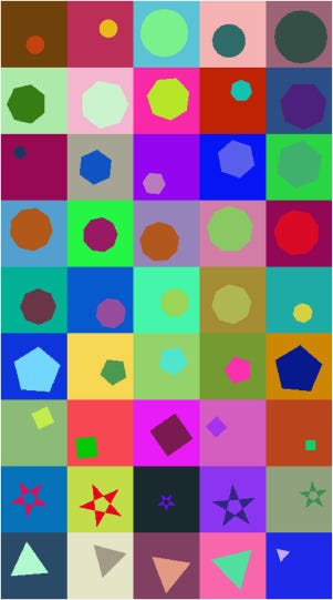
Every good machine learning project begins with a good dataset. For this demonstration, I will utilize the 2D Geometric Shapes Dataset². Created by generating one of 9 different geometric shapes with random orientation, size, and color, the 2D Geometric Shapes Dataset has minimal bias, making it well-suited for deep learning tasks.
Sourced from science direct
Unloading
Let’s begin by downloading the dataset into our working directory and unzipping it.
# Download Dataset and Unzip
download.file(
    "https://data.mendeley.com/public-files/datasets/wzr2yv7r53/files/72256ffc-4020-47e2-8ead-46b40fa15526/file_downloaded",
    destfile = "/kaggle/working/dataset.zip"
)

unzip("dataset.zip")
Once unzipped, the data will be in a folder called “output” containing 90,000 images of size 200 by 200.
Creating a Directory
There is no data directory provided with the data set, so we will need to create one. All the images are in PNG format with a file path similar to the following:
Triangle_6f1d8142–2a58–11ea-8f1b-c869cd928de6.png
We can utilize the fact that the classification of the image is given by the first word before the first underscore to create a data directory.
# Get All Image Paths
images <- list.files(
    "/kaggle/working/output",
    full.names = TRUE
)

# Extract Class Labels
image_labels <- gsub(
    "_.+$",
    "",
    basename(images)
)

# Create Dataset Directory
directory <- data.frame(
    path = images,
    label = image_labels
)
Unique Labels
The {torch} package only works with numeric values, so we will also need to numerically encode our classification labels.
unique_shapes <- c(
  "Circle",
  "Heptagon",
  "Hexagon",
  "Nonagon",
  "Octagon",
  "Pentagon",
  "Square",
  "Star",
  "Triangle"
)
We will refer to each classification label simply as the index of the unique shapes vector. That is, Circle is 1, Heptagon is 2, etc.
Test/Train Split
Now that we have our data set ready to go, let’s create both a training and a testing set. We can do this easily using the {rsample} package. With the rsample::initial_split() function we can randomly split the data and ensure that we have a balanced number of classification labels in each set.
# Test/Train Split
data_split <- rsample::initial_split(
    data = directory,
    strata = label,
    prop = 3/4
)

training_df <- rsample::training(
    data_split
)

testing_df <- rsample::testing(
    data_split
)
We can double check that the spread of class labels is uniformly distributed by using the table() function.
table(training_df$label)

#>  Circle Heptagon  Hexagon  Nonagon  Octagon Pentagon   Square     Star
#>    7500     7500     7500     7500     7500     7500     7500     7500
#>  Triangle
#>    7500
Let’s also create a couple of csv files with the labels and file paths that we will use later.
# Save Label Files
readr::write_csv(
    training_df,
    "/kaggle/working/output/training_labels.csv"
)

readr::write_csv(
    testing_df,
    "/kaggle/working/output/testing_labels.csv"
)
Torch Dataset
Now we are ready for training, right? Well, almost.
The 2D Geometric Shapes Dataset is too large to hold in memory at one time, so, instead, we will need to load the training images into memory in batches.
Creating a single array with all 90,000 images of size 200 by 200 by 3 would take up over 10 billion elements!
But, before we can create our Batch Data Loader, we must first create a Torch Dataset class.
Torch Dataset
The Torch Dataset class is an R6 class that gives instructions to the Batch Data Loader on how to read the images.
Every Torch Dataset class must have an initialization and at least two important methods: .length and .getitem.
It will be of the following form:
# Create the Torch Dataset Class
shapes_dataset <- torch::dataset(
    name = "shapes_dataset",
    initialize = function() {...},
    .getitem = function() {...},
    .length = function() {...}
)- In the
initializefunction we will read in the csv file we created earlier with the paths and labels for each image. - In the
.lengthfunction we will return the number of images in the whole data set. - In the
.getitemfunction we will return a list with two elements,xandy, wherexis a tensor (a type of multi-dimensional array) of the image data andyis the class label also as a tensor of a single numeric value.
Here is what that looks like.
# Create the Torch Dataset
shapes_dataset <- torch::dataset(
    name = "shapes_dataset",
    initialize = function(labels_df) {
        self$labels_df <- readr::read_csv(
          labels_df,
          show_col_types = FALSE
        )
    },
    .getitem = function(i) {
        list(
            x = torch::torch_tensor(
                png::readPNG(
                    self$labels_df$path[i]
                )
            )$view(c(3, 200, 200)),
            y = torch::torch_tensor(
                which(self$labels_df$label[i] == unique_shapes)
            )$squeeze(1)
        )
    },
    .length = function() {
        nrow(self$labels_df)
    }
)
Let’s break that down a bit.
Notice that we read in the labels_df with readr::read_csv() and save it to the variable self$labels_df. This allows it to be accessible by other methods (i.e. functions) in the class.
We also use png::readPNG() to read in the image file path as an array and convert it to a torch tensor with torch::torch_tensor(). We then change its shape from c(200, 200, 3) to c(3, 200, 200) using $view(c(3, 200, 200)) to ensure that the channels are in the first dimension because that is what will be expected by our model.
For y we utilize the unique_shapes vector we created earlier and the which() function from base R to get the index value of the classification label. We wrap this in torch::torch_tensor() and use $squeeze(1) to get rid of the first dimension. Again, this is what will be expected of our model later on.
Lastly, for the .length function we just return the number of rows in the data frame.
Using this Torch Dataset class, we can now create two Torch Datasets: one for the training data and one for the testing data.
training_data <- shapes_dataset("/kaggle/working/output/training_labels.csv")
testing_data <- shapes_dataset("/kaggle/working/output/testing_labels.csv")Check For Correctness
Before moving on, let’s just double check that we set up these data sets correctly. If we run training_data[1]$x we should get back a tensor of size c(3, 200, 200) and if we run length(training_data) we should get back a value equal to the number of rows of the training data csv file we created. You can test for that with the following code.
# Tests to Check
testthat::test_that(
    "dataset was set up correctly",
    {

        # Check Get Item
        testthat::expect_equal(
            dim(training_data[1]$x),
            c(3, 200, 200)
        )

        # Check Length
        testthat::expect_equal(
            length(training_data),
            nrow(readr::read_csv("/kaggle/working/output/training_labels.csv"))
        )
    }
)

#> Test passed 😸
I highly recommend you run these tests yourself because if you don’t, and you get an error later on, you may have a difficult time determining where the error came from.
Data Loaders
Now we are ready to create our Torch Data Loaders. Thankfully, this is pretty straightforward.
training_data_loader <- torch::dataloader(
  training_data,
  batch_size = 128,
  shuffle = TRUE
)

testing_data_loader <- torch::dataloader(
  testing_data,
  batch_size = 128,
  shuffle = FALSE
)
Let’s also run a couple of checks on our Data Loaders to make sure everything is looking good. We can use torch::dataloader_make_iter() and torch::dataloader_next() to run through the first batch and check the dimensions of the data. If everything is correct, we should get a value for the dimensions of x equal to c(batch_size, 3, 200, 200) and y equal to c(batch_size). You can test for that with the following code.
testthat::test_that(
    "dataloader was set up correctly",
    {
        batch <-
            torch::dataloader_next(
                torch::dataloader_make_iter(
                    training_data_loader
                )
            )

        # Check Input Dimensions
        testthat::expect_equal(
            dim(batch$x),
            c(128, 3, 200, 200)
        )

        # Check Target Dimensions
        testthat::expect_equal(
            dim(batch$y),
            c(128)
        )
    }
)
Modeling
Overview
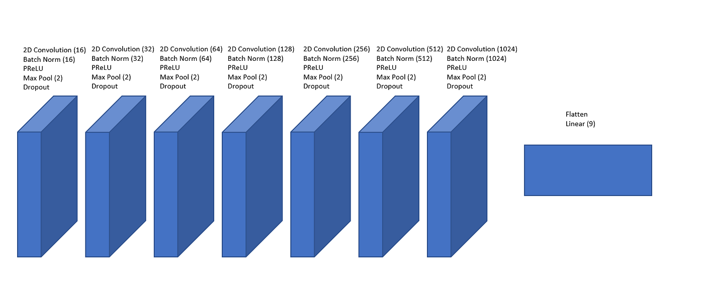
We are finally ready to set up our model architecture and begin training! I tried a lot of different network architectures when working on this article, but the one I chose in the end is the following eight-layer architecture pictured below.
I won’t go into much detail here about what each piece of the model is but if you are interested in knowing more checkout:
A First Go at Image Classification
Model in Code
So, what does this model look like in {torch}? Utilizing the torch::nn_module() class we can set up our neural network. In the initialize method we set up the structure of the network and in the forward function we pass the image to the network and return the result.
# Torch Module Structure
torch::nn_module(
  classname = "",
  initialize = function(){...},
  forward = function(x){...}
)
Our network can be constructed entirely using the torch::nn_sequential() function which allows us to list the transforms of our network in the order we want them to act on the image.
net <- torch::nn_module(
    classname = "net",
    initialize = function(){

        self$net <- torch::nn_sequential(
            torch::nn_conv2d(3, 16, kernel_size = 3, padding = 1, stride = 1),
            torch::nn_batch_norm2d(16),
            torch::nn_prelu(),
            torch::nn_max_pool2d(2),
            torch::nn_dropout(p = 0.2),
            torch::nn_conv2d(16, 32, kernel_size = 3, padding = 1, stride = 1),
            torch::nn_batch_norm2d(32),
            torch::nn_prelu(),
            torch::nn_max_pool2d(2),
            torch::nn_dropout(p = 0.2),
            torch::nn_conv2d(32, 64, kernel_size = 3, padding = 1, stride = 1),
            torch::nn_batch_norm2d(64),
            torch::nn_prelu(),
            torch::nn_max_pool2d(2),
            torch::nn_dropout(p = 0.2),
            torch::nn_conv2d(64, 128, kernel_size = 3, padding = 1, stride = 1),
            torch::nn_batch_norm2d(128),
            torch::nn_prelu(),
            torch::nn_max_pool2d(2),
            torch::nn_dropout(p = 0.2),
            torch::nn_conv2d(128, 256, kernel_size = 3, padding = 1, stride = 1),
            torch::nn_batch_norm2d(256),
            torch::nn_prelu(),
            torch::nn_max_pool2d(2),
            torch::nn_dropout(p = 0.2),
            torch::nn_conv2d(256, 512, kernel_size = 3, padding = 1, stride = 1),
            torch::nn_batch_norm2d(512),
            torch::nn_prelu(),
            torch::nn_max_pool2d(2),
            torch::nn_dropout(p = 0.2),
            torch::nn_conv2d(512, 1024, kernel_size = 3, padding = 1, stride = 1),
            torch::nn_batch_norm2d(1024),
            torch::nn_prelu(),
            torch::nn_max_pool2d(2),
            torch::nn_dropout(p = 0.2),
            torch::nn_flatten(),
            torch::nn_linear(1024 * 1 * 1, 9)
        )

    },
    forward = function(x){
        self$net(x)
    }
)
Just a brief overview of the functions involved:
torch::nn_conv2d()is a convolution which is like a filter that passes over the image to extract out important details.torch::nn_batch_norm2d()is a batch normalization that helps to reduce exploding gradients which can negatively affect training.torch::nn_prelu()is a parametrized rectified linear unit which is the activation function for the network that allows it to fit nonlinear data.torch::nn_max_pool2d()is a max pooling function that grabs the maximum value in a 2 by 2 region and decreases the size of the image by half.torch::nn_dropout()is a function that randomly changes values in the activation to 0 to help prevent overfitting the training data.torch::nn_flatten()is used to flatten the image to a single dimension and prepare it for the dense linear layer.torch::nn_linear()is the final layer that outputs our classification.
Training
Now let's do some training! We will use the {luz} package to help us train the model. We need to specify our loss function and our optimizer function. In this case, we will use cross entropy loss and the Adam optimizer.
A loss function determines how far our predicted label is from the true label and an optimizer function uses the loss to improve the weights in our model.
# Set up Loss and Optimizer
model_setup <-
  luz::setup(
      module = net,
      loss = torch::nn_cross_entropy_loss(),
      optimizer = torch::optim_adam,
      metrics = list(
          luz::luz_metric_accuracy()
      )
  )
Now we can fit the data. Let’s train for 20 epochs (that is, 20 times through the dataset).
# Fit the Data
fitted <-
    luz::fit(
        model_setup,
        training_data_loader,
        epochs = 20,
        verbose = TRUE
    )

#> Epoch 1/20
#> Train metrics: Loss: 2.0029 - Acc: 0.2243
#> Epoch 2/20
#> Train metrics: Loss: 1.2289 - Acc: 0.481
#> Epoch 3/20
#> Train metrics: Loss: 0.7884 - Acc: 0.6618
#> Epoch 4/20
#> Train metrics: Loss: 0.5394 - Acc: 0.7692
#> Epoch 5/20
#> Train metrics: Loss: 0.3822 - Acc: 0.838
#> Epoch 6/20
#> ...
#> Epoch 20/20
#> Train metrics: Loss: 0.0306 - Acc: 0.9893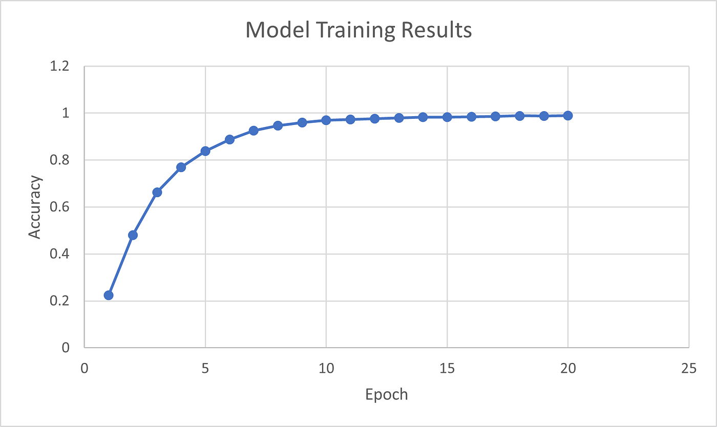
It took 1.2 hours with a GPU accelerator on Kaggle to complete the training. Let’s also save the fitted result.
luz::luz_save(fitted, "/kaggle/working/fitted.rds")Evaluation
So, how’d we do?
Let’s evaluate the accuracy of our model against the validation set.
# Model Accuracy Evaluation
luz::evaluate(
    fitted,
    testing_data_loader
)

#> A `luz_module_evaluation`
#> ── Results ─────────────────────────────────────────────────────────────────────
#> loss: 0.0156
#> acc: 0.9945
99.5% accuracy. Nice!
But what did we get wrong?
Let’s gather up the model predictions …
predictions <- predict(
    fitted,
    testing_data_loader
)

prediction_classes <- torch::as_array(
    predictions$argmax(2)$to(device = "cpu")
)

prediction_df <- data.frame(
    label = testing_df$label,
    truth = match(testing_df$label, unique_shapes),
    estimate = prediction_classes
)

head(prediction_df)

#> A data.frame: 6 × 3
#> label truth estimate
#> <chr> <int> <int>
#> Circle  1     1
#> Circle  1     1
#> Circle  1     1
#> Circle  1     1
#> Circle  1     1
#> Circle  1     1
… and compare the accuracy across the nine shapes.
dplyr::summarize(
    dplyr::group_by(
        prediction_df,
        label
    ),
    perc_correct = sum(truth == estimate)/length(truth)
)

#> A tibble: 9 × 2
#> label  perc_correct
#> <chr>     <dbl>
#> Circle    0.9964
#> Heptagon  0.9948
#> Hexagon   0.9948
#> Nonagon   0.9844
#> Octagon   0.9896
#> Pentagon  0.9972
#> Square    0.9960
#> Star      0.9976
#> Triangle  1.0000
Wow! 100% percent accuracy on the triangle. That makes sense, considering it is a very unique compared to the other shapes. On the flip side it seems like the model struggled the most on identifying nonagons and octagons. Could this be because they look like circles? Let’s take a look at what the model thought.
dplyr::summarize(
    dplyr::group_by(
        dplyr::filter(prediction_df, label == "Nonagon"),
        estimate
    ),
    num_guesses = length(estimate)
)

#> A tibble: 6 × 2
#> estimate num_guesses
#> <int> <int>
#>   1    27
#>   2    2
#>   4    2461
#>   5    5
#>   6    1
#>   9    4
2461 of the 2500 Nonagon images were classified as Nonagon, 5 as Octagon, and 27 as Circle! So, it seems our hunch was correct.
Conclusion
We made it! Thank you for reading and I hope you enjoyed it! Until the next one.
Citations
[1] “Torch for R.” Torch for R, torch.mlverse.org/. Accessed 8 July 2023.
[2] Korchi, Anas El, and Youssef Ghanou. “2D Geometric Shapes Dataset — for Machine Learning and Pattern Recognition.” Data in Brief, vol. 32, 25 July 2020, https://doi.org/10.1016/j.dib.2020.106090.
- This blog post was originally published at: https://blog.devgenius.io