Despite a booming adoption of machine learning in making critical decisions, many machine learning models remain black boxes. Here trust and ethical challenges of using machine learning in making decisions come into the picture. Because the real-world consequences of wrong prediction can be expensive. In 2017, a lawsuit was filed against three US-based companies responsible for designing and developing an automated computer system which was used by Michigan government unemployment agency and made 20,000 false fraud accusations. A good boss will also question his data team why the company should be making these critical business decisions. In order not to blindly trust machine learning models, the need for understanding model’s behaviors, the decisions it makes, and any associated potential pitfalls is high on the agenda.
Model interpretability — Post hoc explanation technique
A commonly accepted phenomenon in data science community and literature (Johansson, Ulf, et al., 2011; Choi, Edward, et al., 2016, etc.) is that there is a trade-off between model accuracy and interpretability. At times
when you have a very large potentially complicated dataset, the use of complex models such as deep neural nets and random forests often achieve higher performance, but lower interpretability. In contrast, simpler models, such as linear or logistic regression just to name a few, often offer lower performance but higher interpretability. This is where post hoc explanation techniques emerge and become a game changer in machine learning literature.
Traditional statistical methods use a hypothesis-driven approach, which means that we construct the assumptions and verify hypotheses by training the models. Post hoc techniques, on the contrary, are set-up techniques which are applied “after the event”- after model training. So the idea people come up with is to first build complex models for making decisions and then explain them using simpler models. In other words, constructing complex model first and assumptions will come later. Some examples of post hoc explanation techniques include LIME, SHAP, Anchor, MUSE amongst others. My point of discussion in this article will be explaining what LIME is and how it works using a step-by-step guide with Python codes as well as the good and the ugly associated with LIME.
So what the heck is LIME and how does it work?
LIME is the abbreviation for Local Interpretable Model-agnostic Explanations. In essence, LIME is Model-agnostic, meaning that it can be applied to ANY models based on the assumption that every complex model is a black-box. By interpretable manner, it implies that LIME will be able to explain how the model behaves, which features it picks up and what kinds of interactions between them take place to drive the predictions. Last but certainly not least, LIME is observation specific, meaning that it tries to understand features that influence the black-box model around a single instance of interest. The rationale behind LIME is that as global model interpretability is very difficult to achieve in reality, it is far simpler to approximate a black-box model by a simple model locally.
In practice, the decision boundary of a black-box model can look very complex. In the figure below, the decision boundary of a black-box model is represented by the blue-pink background, which seems too complex to be accurately approximated by a linear model.
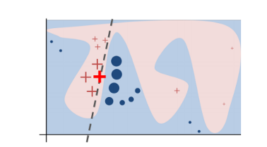
Decision boundary of blackbox model.
However, studies (Baehrens, David, et al. (2010), Laugel et al., 2018 etc.) have shown that when you zoom in and look at a small enough neighborhood (bear with me, I will discuss what it means a meaningful neighborhood in the next session), no matter how complex the model is at a global level, the decision boundary at a local neighborhood can be a much more simpler, can in fact be even linear. For instance, the probability of someone having a cancer may be nonlinearly dependent on his age. But if you are looking at only a small group of people who are more than 70 so to say, there is a likelihood that for that subset of the population, the risk of having cancer is linearly correlated with increase in age.
That being said, what LIME does is to go on a very local level and get to a point where it becomes so local that a linear model is powerful enough to explain the behavior of the original black-box model at the local level and it will be highly accurate on that locality (in the neighborhood of the observation we want to explain). In the example (Figure 1), the bold red cross is the instance being explained. LIME will generate new instances by sampling a neighborhood around this selected instance, applying the original black-box model on that neighborhood to generate the corresponding predictions, and weighting those generated instances by their distances to the instance being explained.
In this obtained dataset (which includes the generated instances, the corresponding predictions and the weights), LIME trains an interpretable model (e.g weighted linear model, decision trees) which captures the behaviors of the complex model in that neighborhood. The coefficients of that local linear model will serve as the explanators and tell us which features drive the prediction to one way or the other. In Figure 1, the dashed line is the behaviour of the black-box model in a specific locality which can be explained by a linear model and the explanation is considered faithful in that locality.
#lime #black-box #machine-learning #data-science