Linear regression is probably the most simple machine learning algorithm. It is very good for starters because it uses simple formulas. So, it is good for learning machine-learning concepts. In this article, I will try to explain the multivariate linear regression step by step.

Concepts and Formulas

Linear regression uses the simple formula that we all learned in school:

Y = C + AX

Just as a reminder, Y is the output or dependent variable, X is the input or the independent variable, A is the slope, and C is the intercept.

For the linear regression, we follow these notations for the same formula:

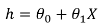
If we have multiple independent variables, the formula for linear regression will look like:

Here, ‘h’ is called the hypothesis. This is the predicted output variable. Theta0 is the bias term and all the other theta values are coefficients. They are initiated randomly in the beginning, then optimized with the algorithm so that this formula can predict the dependent variable closely.

Cost Function and Gradient Descent

When theta values are initiated in the beginning, the formula is not trained to predict the dependent variable. The hypothesis is far away from the original output variable ‘Y’. This is the formula to estimate the cumulative distance of all the training data:

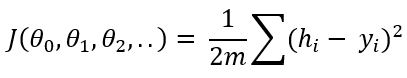
This is called the cost function. If you notice, it deducts y(the original output) from the hypothesis(the predicted output), takes the square to omit the negativity, sum up and divide by 2 times m. Here, m is the number of training data. You probably can see that cost function is the indication of the difference between the original output and the predicted output. The idea of a machine learning algorithm is to minimize the cost function so that the difference between the original output and the predicted output is closer. To achieve just that, we need to optimize the theta values.

Here is how we update the theta values. We take the partial differential of the cost function with respect to each theta value and deduct that value from the existing theta value,

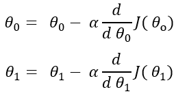
Here, alpha is the learning rate and it is a constant. I am not showing the same formula for all the theta values. But It is the same formula for all the theta values. After the differentiation, the formula comes out to be:

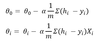
This is called gradient descent.

Implementation of the Algorithm Step by Step

The dataset I am going to use is from Andre Ng’s machine learning course in Coursera. I will provide the link at the bottom of this page. Please feel free to download the dataset and practice with this tutorial. I encourage you to practice with the dataset as you read if this is new to you. That is the only way to understand it well.

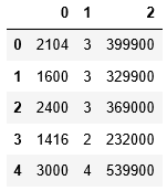
In this dataset, there are only two variables. But I developed the algorithm for any number of variables. If you use the same algorithm for 10 variables or 20 variables, it should work as well. I will use Numpy and Pandas library in Python. All these rich libraries of Python made the machine learning algorithm a lot easier. Import the packages and the dataset:

import pandas as pd
import numpy as np

df = pd.read_csv('ex1data2.txt', header = None)
df.head()

#machine-learning #data-science #machine-intelligence #python