1.0 Introduction to PM
When it comes to dealing with machines that require periodic maintenance, there are generally three possible outcomes.
One, you can maintain a machine too frequently. In other words, the machine gets maintenance when it is not required. In this scenario, you are throwing money out the window, wasting resources providing unnecessary maintenance. For example, you could change the oil in your car every single day. This is clearly not optimal, and you will waste a lot of money on unnecessary maintenance.
Two, you don’t maintain your machine frequently enough. Failing to maintain a machine means that the machine will break while operating. Here, the costs could be substantial. Not only do you have the repair costs, but also costs associated with lost production. If a machine on the assembly line goes down, the line cannot produce anything. No production means lost profit. Also, you will incur legal and medical costs if injuries occurred as a result of the failure.
Three, a machine is maintained when it needs maintenance. This is obviously the better alternative of the three. Note, that that there is still a cost associated with timely maintenance.
So, we need to maintain machines when they need maintenance, right? Unfortunately, this is easier said than done. Fortunately, we can use predictive maintenance (PM) to predict when machines need maintenance.
I should also mention that most machines come with manufacturer recommendations on maintenance. The problem with manufacturer recommendations is that they represent an average. For example, cars on average need an oil change every 3,000 miles, but how frequently does your car need an oil change? It may be more or less than 3,000 miles depending on several factors including where your drive, how you drive and how frequently you drive.
Predictive maintenance (PM) can tell you, based on data, when a machine requires maintenance. An effective PM program will minimize under and over maintaining your machine. For a large manufacturer with thousands of machines, being precise on machine maintenance can save millions of dollars every year.
In this article, I will examine a typical Predictive Maintenance (PM) use case. As I walk through this example, I will describe some of the issues that arise with PM problems and suggest ways to solve them.
An important note about the data used in this exercise. It is completely fake. I created the data based on my experience of dealing with these types of problems. Although it is completely fake, I believe the data and use case are very realistic and consistent with many real PM problems.
2.0 Use case
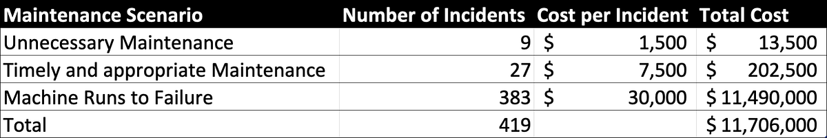
The firm in our use case provided a sample of data that includes 419 machines that failed over a two year period. They spent about 11.7M dollars on maintenance, most of which came from running machines until failure.
Here is a summary of the maintained or repaired machines over the last two years.

From the data above, it currently costs the firm about $28,000 per failed or maintained machine. Our goal is to lower this cost.
In the chart above, Timely Maintenance costs more than Unnecessary Maintenance. There is a good reason for this. For this machine, Unnecessary Maintenance means that that machine was moved off-line and and checked but the part in question showed insufficient wear to replace. Because parts were not replaced, there are no material costs, only labor.
Note that this company does very little predictive maintenance. Most of the time they just run the machines to failure. Also note that these machines will break in four to eight years if they don’t receive maintenance. When they break, the must be pulled off-line and repaired.
Our goal is to show the firm how a Predictive Maintenance program can save them money. To do this we will build a predictive model that predicts machine failure within 90 days of failure. **Note that an appropriate failure window will always depend on the context of the problem. **If a machine breaks without maintenance in 6 months, a 3 month window makes no sense. Here, where a machine will run between 4 to 6 years without maintenance, a 90 day window is reasonable.
Our objective is to develop a solution that will lower the costs of failure. Again, it currently costs the firm about 28,000 per machine. We will attempt to lower this cost.
3.0 Setting up the Environment and Previewing the Data
The first step in solving the problem at hand is to ensure that we have the appropriate libraries installed in our Jupyter Notebook. In this exericise, I will be using python code in a Jupyter notebook inside Watson Studio from IBM.
!pip install --upgrade numpy
!pip install imblearn --upgrade
!pip install plotly --upgrade
!pip install chart-studio --upgrade
import chart_studio.plotly as py
import plotly.graph_objs as go
import numpy.dual as dual
import plotly as plotly
import pandas as pd
from botocore.client import Config
import ibm_boto3
import numpy as np
import numpy.dual as dual
from imblearn.over_sampling import SMOTE
from imblearn.over_sampling import SMOTENC
from sklearn import metrics
from sklearn.preprocessing import LabelEncoder
import xgboost as xgb
from xgboost.sklearn import XGBClassifier
import types
import pandas as pd
from botocore.client import Config
import ibm_boto3
def __iter__(self): return 0
Next, we will import our data from github to the Jupyter environment.
#Remove the data if you run this notebook more than once
!rm equipment_failure_data_1.csv

#import first half from github
!wget https://raw.githubusercontent.com/shadgriffin/machine_failure/master/equipment_failure_data_1.csv
# Convert csv to pandas dataframe
pd_data_1 = pd.read_csv("equipment_failure_data_1.csv", sep=",", header=0)
#Remove the data if you run this notebook more than once
!rm equipment_failure_data_2.csv
#Import the second half from github
!wget https://raw.githubusercontent.com/shadgriffin/machine_failure/master/equipment_failure_data_2.csv
# convert to pandas dataframe
pd_data_2 = pd.read_csv("equipment_failure_data_2.csv", sep=",", header=0)
#concatenate the two data files into one dataframe
pd_data=pd.concat([pd_data_1, pd_data_2])
Now that we have the data imported into a Jupiter Notebook, we can explore it. Here is meta data explaining all of the fields in the data set.
ID — ID field that represents a specific machine.
DATE — The date of the observation.
REGION_CLUSTER — a field that represents the region in which the machine is located.
MAINTENANCE_VENDOR — a field that represents the company that provides maintenance and service to the machine.
MANUFACTURER — the company that manufactured the equipment in question.
WELL_GROUP — a field representing the type of Machine.
EQUIPMENT_AGE — Age of the machine, in days.
S15 — A Sensor Value.
S17 — A Sensor Value.
S13 — A Sensor Value.
S16 — A Sensor Value.
S19 — A Sensor Value.
S18 — A Sensor Value.
S8 — A Sensor Value.
EQUIPMENT_FAILURE — A ‘1’ means that the equipment failed. A ‘0’ means the equipment did not fail.
Our first goal in this exercise is to build a model that predicts equipment failure. In other words, we will use the other variables in the data frame to predict EQUIPMENT_FAILURE.
Now we will walk through the data, gaining an understanding of what kind of data set we are dealing with.
pd_data.shape

The data has 307,751 rows and 16 columns
xxxx = pd.DataFrame(pd_data.groupby(['ID']).agg(['count']))
xxxx.shape
There are 421 machines in the data set

xxxx = pd.DataFrame(pd_data.groupby(['DATE']).agg(['count']))
xxxx.shape
There are 731 unique dates in the data set

So, if we have 421 machines and 731 unique dates, we should have 307,751 total records. Based on the .shape command a few steps ago, we have one record per machine per date value. There are no duplicates in the data frame.
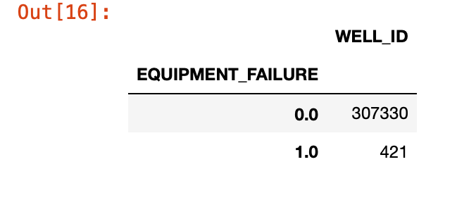
Now let’s examine the dependent variable in more detail. It appears that out of 307,751 records, we only have 421 failures. This corresponds to a failure rate of about .14%. In other words, for every failure you have over 700 non-failures. This data set is very unbalanced. Later in this article I will use a few techniques to mitigate the impact of a small number of observed failures.
xxxx = pd.DataFrame(pd_data.groupby(['EQUIPMENT_FAILURE'])['ID'].agg('count'))
xxxx
4.0 Feature Engineering with a Panel Data Set
Next, we can start to transform our data so that it is ready for a machine learning model. Specifically, we will create running summaries of the sensor values. Running summaries of sensor values are often useful in predicting equipment failure. For example, if a temperature gauge indicates a machine is warmer than average for the last 5 days, it may indicate something is wrong.
Remember that we are working with a panel data set. That is, we have multiple machines measured over two years. As we create our running summaries, we have to make sure that our summaries do not include more than one machine. For example, if we create a 10 day moving average, we do not want the first 9 days of a machine to include values from the previous machine.
Note, that I create twenty one day summaries in this example. That works in this use case, but with other use cases it could be advantageous to use more or different time intervals.
First, define your feature window. This the window by which we will aggregate our sensor values. Next, convert dates from character to date in the pandas data frame.
feature_window=21
pd_data['DATE'] = pd.to_datetime(pd_data['DATE'])
Create a new field called “flipper” that indicates when a the id changes as the data is sorted by ID and DATE in ascending order. We will use this in a few other transformations.
pd_data=pd_data.sort_values(by=['ID','DATE'], ascending=[True, True])

pd_data['flipper'] = np.where((pd_data.ID != pd_data.ID.shift(1)), 1, 0)
Calculate the number of days since the first day a machine appears to the current day. This field will be called “TIME_SINCE_START” Also create a variable called “too_soon”. When “too_soon” is equal to 1 we have less than 21 days (feature_window) of history for the machine.
We will use these new variables to create a running mean, median, max and min. Also, we will need to augment the running statistics for records that have less than five days of history.
dfx=pd_data

#Select the first record of each machine
starter=dfx[dfx['flipper'] == 1]
starter=starter[['DATE','ID']]
#rename date to start_date
starter=starter.rename(index=str, columns={"DATE": "START_DATE"})
#convert START_DATE to date
starter['START_DATE'] = pd.to_datetime(starter['START_DATE'])
#Merge START_DATE to the original data set
dfx=dfx.sort_values(by=['ID', 'DATE'], ascending=[True, True])
starter=starter.sort_values(by=['ID'], ascending=[True])
dfx =dfx.merge(starter, on=['ID'], how='left')
# calculate the number of days since the beginning of each well.
dfx['C'] = dfx['DATE'] - dfx['START_DATE']
dfx['TIME_SINCE_START'] = dfx['C'] / np.timedelta64(1, 'D')
dfx=dfx.drop(columns=['C'])
dfx['too_soon'] = np.where((dfx.TIME_SINCE_START < feature_window) , 1, 0)
Create a running mean, max, min and median for the sensor variables.
dfx['S5_mean'] = np.where((dfx.too_soon == 0),(dfx['S5'].rolling(min_periods=1, window=feature_window).mean()) , dfx.S5)
dfx['S5_median'] = np.where((dfx.too_soon == 0),(dfx['S5'].rolling(min_periods=1, window=feature_window).median()) , dfx.S5)
dfx['S5_max'] = np.where((dfx.too_soon == 0),(dfx['S5'].rolling(min_periods=1, window=feature_window).max()) , dfx.S5)
dfx['S5_min'] = np.where((dfx.too_soon == 0),(dfx['S5'].rolling(min_periods=1, window=feature_window).min()) , dfx.S5)
dfx['S13_mean'] = np.where((dfx.too_soon == 0),(dfx['S13'].rolling(min_periods=1, window=feature_window).mean()) , dfx.S13)
dfx['S13_median'] = np.where((dfx.too_soon == 0),(dfx['S13'].rolling(min_periods=1, window=feature_window).median()) , dfx.S13)
dfx['S13_max'] = np.where((dfx.too_soon == 0),(dfx['S13'].rolling(min_periods=1, window=feature_window).max()) , dfx.S13)
dfx['S13_min'] = np.where((dfx.too_soon == 0),(dfx['S13'].rolling(min_periods=1, window=feature_window).min()) , dfx.S13)
dfx['S15_mean'] = np.where((dfx.too_soon == 0),(dfx['S15'].rolling(min_periods=1, window=feature_window).mean()) , dfx.S15)
dfx['S15_median'] = np.where((dfx.too_soon == 0),(dfx['S15'].rolling(min_periods=1, window=feature_window).median()) , dfx.S15)
dfx['S15_max'] = np.where((dfx.too_soon == 0),(dfx['S15'].rolling(min_periods=1, window=feature_window).max()) , dfx.S15)
dfx['S15_min'] = np.where((dfx.too_soon == 0),(dfx['S15'].rolling(min_periods=1, window=feature_window).min()) , dfx.S15)
dfx['S16_mean'] = np.where((dfx.too_soon == 0),(dfx['S16'].rolling(min_periods=1, window=feature_window).mean()) , dfx.S16)
dfx['S16_median'] = np.where((dfx.too_soon == 0),(dfx['S16'].rolling(min_periods=1, window=feature_window).median()) , dfx.S16)
dfx['S16_max'] = np.where((dfx.too_soon == 0),(dfx['S16'].rolling(min_periods=1, window=feature_window).max()) , dfx.S16)
dfx['S16_min'] = np.where((dfx.too_soon == 0),(dfx['S16'].rolling(min_periods=1, window=feature_window).min()) , dfx.S16)
dfx['S17_mean'] = np.where((dfx.too_soon == 0),(dfx['S17'].rolling(min_periods=1, window=feature_window).mean()) , dfx.S17)
dfx['S17_median'] = np.where((dfx.too_soon == 0),(dfx['S17'].rolling(min_periods=1, window=feature_window).median()) , dfx.S17)
dfx['S17_max'] = np.where((dfx.too_soon == 0),(dfx['S17'].rolling(min_periods=1, window=feature_window).max()) , dfx.S17)
dfx['S17_min'] = np.where((dfx.too_soon == 0),(dfx['S17'].rolling(min_periods=1, window=feature_window).min()) , dfx.S17)
dfx['S18_mean'] = np.where((dfx.too_soon == 0),(dfx['S18'].rolling(min_periods=1, window=feature_window).mean()) , dfx.S18)
dfx['S18_median'] = np.where((dfx.too_soon == 0),(dfx['S18'].rolling(min_periods=1, window=feature_window).median()) , dfx.S18)
dfx['S18_max'] = np.where((dfx.too_soon == 0),(dfx['S18'].rolling(min_periods=1, window=feature_window).max()) , dfx.S18)
dfx['S18_min'] = np.where((dfx.too_soon == 0),(dfx['S18'].rolling(min_periods=1, window=feature_window).min()) , dfx.S18)
dfx['S19_mean'] = np.where((dfx.too_soon == 0),(dfx['S19'].rolling(min_periods=1, window=feature_window).mean()) , dfx.S19)
dfx['S19_median'] = np.where((dfx.too_soon == 0),(dfx['S19'].rolling(min_periods=1, window=feature_window).median()) , dfx.S19)
dfx['S19_max'] = np.where((dfx.too_soon == 0),(dfx['S19'].rolling(min_periods=1, window=feature_window).max()) , dfx.S19)
dfx['S19_min'] = np.where((dfx.too_soon == 0),(dfx['S19'].rolling(min_periods=1, window=feature_window).min()) , dfx.S19)
Another useful transformation is to look for sudden spikes in sensor values. This code creates an value indicating how far the current value is from the immediate norm.
dfx['S5_chg'] = np.where((dfx.S5_mean == 0),0 , dfx.S5/dfx.S5_mean)

dfx['S13_chg'] = np.where((dfx.S13_mean == 0),0 , dfx.S13/dfx.S13_mean)
dfx['S15_chg'] = np.where((dfx.S15_mean==0),0 , dfx.S15/dfx.S15_mean)
dfx['S16_chg'] = np.where((dfx.S16_mean == 0),0 , dfx.S16/dfx.S16_mean)
dfx['S17_chg'] = np.where((dfx.S17_mean == 0),0 , dfx.S17/dfx.S17_mean)
dfx['S18_chg'] = np.where((dfx.S18_mean == 0),0 , dfx.S18/dfx.S18_mean)
dfx['S19_chg'] = np.where((dfx.S19_mean == 0),0 , dfx.S19/dfx.S19_mean)
#predictive-maintenance #data-science #machine-learning #equipment-failure #python #deep learning