Contents

1. Gradient descent advanced optimization techniques
2. Autoencoders
3. Dropout
4. Pruning

Gradient descent advanced optimization techniques:

In this post we will cover a few advanced techniques namely,

Momentum ,Adagrad, RMSProp ,Adam etc

A machine learning model can contain millions of parameters or dimensions. Therefore the cost function has to be optimized over millions of dimensions.

The goal is to obtain a global minimum of the function which will give us the best possible values to optimize our evaluation metric with the given parameters.

The odds of obtaining a local minima inmost of the dimensions a high dimensional space are low , we are much more likely to encounter saddle points.

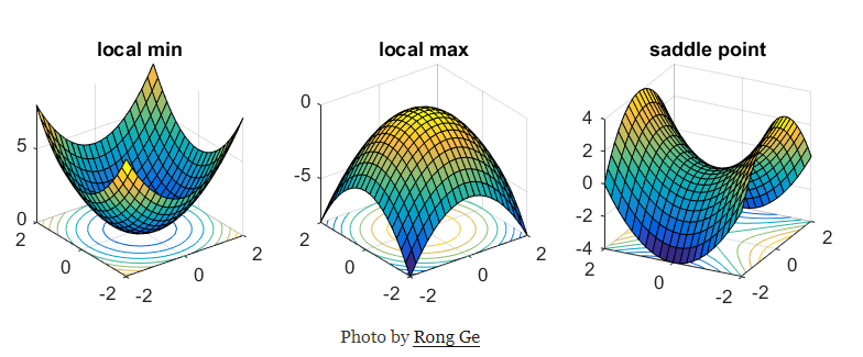
**Saddle Points:**a point at which a function of two variables has partial derivatives equal to zero but at which the function has neither a maximum nor a minimum value.

In mathematics, a saddle point is a point on the surface of the graph of a function where the slopes(derivatives) in orthogonal directions are all zero (a crtitical point), but which is not a local extremum of the function. An example of a saddle point is when there is a critical point with a relative minimum along one axial direction (between peaks) and at a relative maximum along the crossing axis.

Saddle points can drastically slow down optimization process , In the diagrams shown below the stochastic gradient descent converges prematurely to a value which is below optimum. The other points are different optimization techniques

In gradient descent we take a step along the gradient in each dimension. In the first animation,using SGD we get stuck in the local minima of one dimension , while we are also at the local maxima of another dimension( Gradient is close to zero)

Because our step size in a given dimension is determined by the gradient value, we’re slowed down in the presence of local optima.

#rmsprop #adam #momentum #autoencoder #dropout