Introduction
Support Vector Classifiers (SVC) and Logistic Regression (LR) can align to the extent that they can be the exact same thing. Understanding when SVC and LR are exactly the same will help with the intuition of how exactly they are different.
Logistic Regression (LR) is a probabilistic classification model using the sigmoid function, whereas Support Vector Classifiers (SVC) are a more geometric approach that maximise the margins to each class. They are similar in that they both can divide the feature space with a decision boundary. I often hear the question about the difference between these two machine learning algorithms, and the answer to this always focuses on the precise details of the log-odds generalised linear model in LR and the maximum-margin hyperplane, soft and hard margins of SVC.
**I think it is useful to look at the opposite case: **when are LR and SVC exactly the same?!
The answer: when exclusively using binary features with a binary outcome predictor, a LR model without regularisation and SVC with linear kernel.
Let’s very briefly review LR and SVC then give the example to show these decision boundaries can be exactly the same.
Logistic Regression
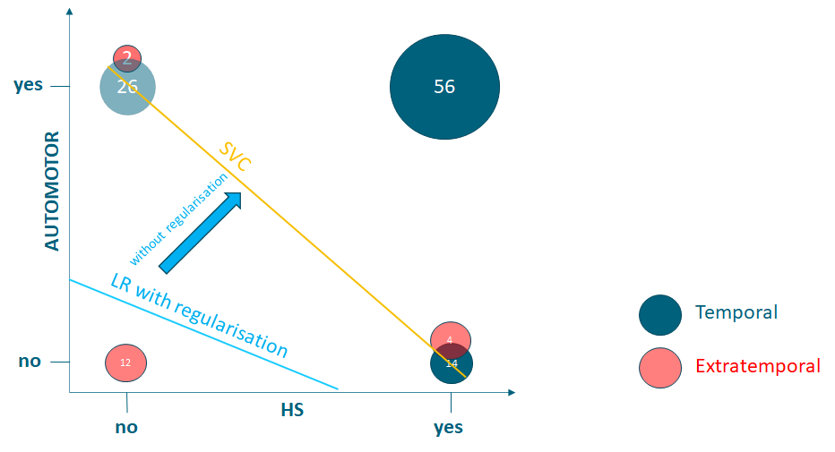
Let’s give the example of trying to determine if epileptic seizures arise from the temporal lobe in the brain, or elsewhere (extratemporal), using what the seizure looks like (semiology) and what we find on a brain scan.
**Features: **What happens during a seizure e.g. arm shaking or fiddling with fingers (Semiology) and an abnormality on brain scan called hippocampal sclerosis (HS) (all features are binary)
**Target predictor: **are seizures coming from the temporal lobe? (binary)
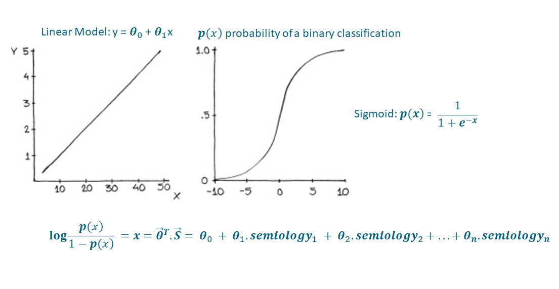
Figure 1: Logistic Regression Summary
Logistic regression is a classification model, despite its name. The basic idea is to give the model a set of inputs, x, which can be multidimensional, and get a probability as seen on the right-panel image of Figure 1. This can be useful when we want the probability of a binary target between 0 and 1, as opposed to a linear regression (left panel of Figure 1). If we rearrange the sigmoid function above and solve for x, we arrive at the logit function (aka log-odds) which is a clear generalised linear model (bottom equation in Figure 1).
LR is all about finding the optimal (theta) coefficients in this model, such that the overall error (cost function) is minimised, by gradient descent (Figure 2):
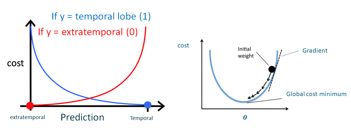
Figure 2: LR Cost Function using the example of temporal vs extratemporal seizure foci as target predictor. The image on the left is represented by the cost = -y.log(p(x)) — (1-y).log(1-p(x)). Where y is the true binary label. The image on the right shows gradient descent using partial derivates of the coefficients.
Add to the cost function a regularisation parameter (1/C) (which multiplies the sum of the squares of the coefficients):
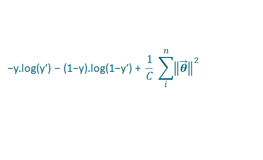
Equation 1: Cost function with L2 regularisation for LR. L2 means the theta coefficients are squared. y is the true binary label. y’ is the probability of the label as predicted by the model: p(x).
Sklearn has a LogisticRegression() classifier, the default regularisation parameters are penalty=L2 and C=1. This term penalises overfitting. Unfortunately, it can also result in underfitting in the special case below, resulting in worse cross-validated performance. But when this regularisation is removed, for the special case below, we will see that it merges into being the same model as a SVC.
#logistic-regression #machine-learning #support-vector-machine #classification-models #regularization #deep learning