In this publication I will write about the mathmatics behind the simplest 2D Convolutional Neural Network (CNN), I’ll try to make a connection to the Multi Layer Perceptron (MLP) that I wrote about in my last publication. I’ll present a model architecture, forward and back propagation calculations and finally show some other techniques that are widelly used in modern CNNs.

The CNN was implemented as a model that could handle images in a more efficient way than the MLP. Through the usage of kernel masks containing weights, the networks find characteristic patterns in the input images like edges, corners, circles, etc. If the network is complex enough it even may find more detailed structures like whole faces, cars, animals and so on.

The kernel masks extract features from the inputs by sliding over them. Each mask operates a matrix multiplication with the input matrix around the values it covers. For better understanding, the next image represents a kernel mask with shape 2 x 2 sliding over an input image of 3 x 3 pixels, our input:

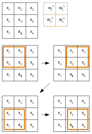
As you can see, the mask goes from left to right and top to bottom.

I use a 3 x 3 instance of an image for simplicity, depite, in general, images being of greater size.

Kernel masks can be whichever size we want. Generally 3 x 3 masks provide good results, but can be optimized like any other hyperparameter.

Let’s say we choose to have a filter of three masks. The results are three net input matrices that are then activated by an activation funtion, we’ll use sigmoid (not represented bellow).

#pooling #batch-normalization #mathematics #convolutional-network #neural networks