This is Part 4 of our ongoing series on NumPy optimization. In Parts 1 and 2 we covered the concepts of vectorization and broadcasting, and how they can be applied to optimize an implementation of the K-Means clustering algorithm. Next in the cue, Part 3 covered important concepts like strides, reshape, and transpose in NumPy. In this post, Part 4, we’ll cover the application of those concepts to speed up a deep learning-based object detector: YOLO.

Part 3 outlined how various operations like reshape and transpose can be used to avoid unnecessary memory allocation and data copying, thus speeding up our code. In this part, we will see it in action.

We will focus particularly on a specific element in the output pipeline of our object detector that involves re-arranging information in memory. Then we’ll implement a naïve version where we perform this re-arranging of information by using a loop to copy the information to a new place. Following this we’ll use reshape and transpose to optimize the operation so that we can do it without using the loop. This will lead to considerable speed up in the FPS of the detector.

So let’s get started!

Understanding the problem statement

The problem that we are dealing with here arises due to, yet again, nested loops (no surprises there!). I encountered it when I was working on the output pipeline of a deep learning-based object detector called YOLO (You Only Look Once) a couple of years ago.

Now, I don’t want to digress into the details of YOLO, so I will keep the problem statement very limited and succinct. I will describe enough so that you can follow along even if you have never even heard of object detection.

YOLO uses a convolutional neural network to predict objects in an image. The output of the detector is a convolutional feature map.

In case the couple of lines above sound like gibberish, here’s a simplified version. YOLO is a neural network that will output a convolutional feature map, which is nothing but a fancy name for a data structure that is often used in computer vision (just like Linked Lists, dictionaries, etc.).

A convolutional feature map is essentially a spatial grid with multiple channels. Each channel contains information about a specific feature across all locations in the spatial grid. In a way, an image can also be defined as a convolutional feature map, with 3 channels describing intensities of red, green, and blue colors. A 3-D image, where each channel contains a specific feature.

Let’s say we are trying to detect objects in an image containing a Rail engine. We give the image to the network and our output is something that looks like the diagram below.

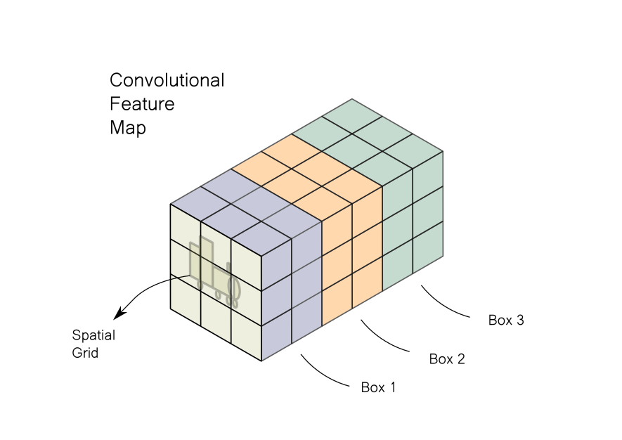
The image is divided into a grid. Each cell of the feature map looks for an object in a certain part of the image corresponding to each grid cell. Each cell contains data about 3 bounding boxes which are centered in the grid. If we have a grid of say 3 x 3, then we will have data of 3 x 3 x 3 = 27 such boxes. The output pipeline would filter these boxes to leave the few ones containing objects, while most of others would be rejected. The typical steps involved are:

1. Thresholding boxes on the basis of some score.
2. Removing all but one of the overlapping boxes that point to the same object.
3. Transforming data to actual boxes that can be drawn on an image.

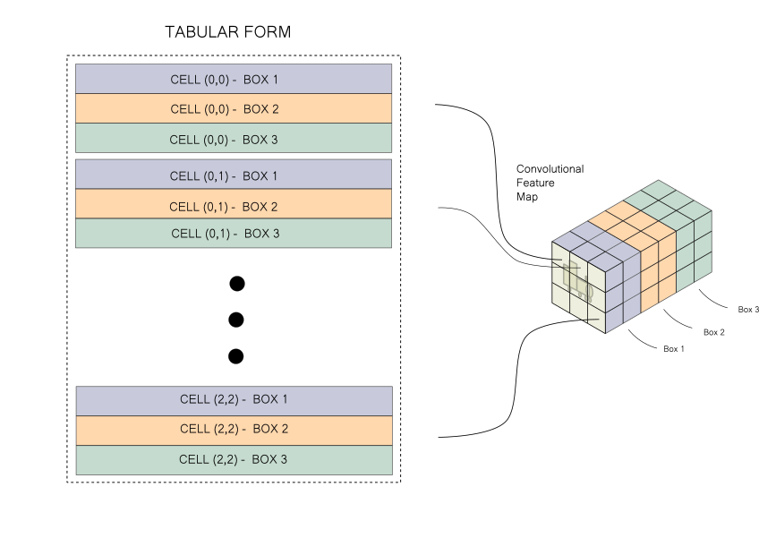
However, given the way information is stored in a convolutional feature map, performing the operations highlighted above can lead to messy code (for more details, refer to Part 4 of the YOLO series). To make the code easier to read and manage, we would like to take the information stored in a convolutional feature map and rearrange it to a tabular form, like the one below.

And that’s the problem! We simply need to rearrange information. That’s it. No need to go further into YOLO! So let’s get to it.

Setting up the experiment

For the purposes of this experiment, I have provided the pickled convolutional feature map which can be downloaded from here.

We first load the feature map into our system using pickle.

import pickle 
conv_map = pickle.load(open("conv_map.pkl", "rb"))

The convolutional neural network in PyTorch, one of most widely-used deep learning libraries, is stored in the [B x C x H x W] format where B is batch size, C is channel, and H and W are the dimensions. In the visualization used above, the convolutional map was demonstrated with format [H W C], however using the [C H W] format helps in optimizing computations under the hood.

The pickled file contains a NumPy array representing a convolutional feature map in the [B C H W] format. We begin by printing the shape of the loaded array.

print(conv_map.shape)
#output -> (1, 255, 13, 13)

Here the batch size is 1, the number of channels is 255, and the spatial dimensions are 13 x 13. 255 channels correspond to 3 boxes, with information for each box represented by 85 floats. We want to create a data structure where each row represents a box and we have 85 columns representing this information.

#numpy #deep-learning #developer #data-science