Recently there was a nice article on Medium explaining why data scientists should start using Spark and Scala instead of Pandas. Although the article contains many valid points, I propose a more differentiated view, which is also reflected in my personal work where I use both, but for different kinds of tasks.
Whenever I gave a training for PySpark to Data Scientists, I was always asked if they should stop using Pandas from now on altogether, or when to prefer which of the two frameworks Pandas and Spark. For answering this question you need to understand each tools strengths and limitations and you should understand that both frameworks have been developed to solve similar problems but each with a different focus.
This is the first part of a small series for comparing Spark and Pandas.
- Spark vs Pandas, part 1 — Pandas
- Spark vs Pandas, part 2 — Spark
- Spark vs Pandas, part 3 — Programming Languages
- Spark vs Pandas, part 4 — Shootout and Recommendation
What to Expect
I will present both frameworks Pandas and Spark and discuss their strengths and weaknesses to set the ground for a fair comparison. Originally I wanted to write a single article on this topic, but it continued to grow until I decided to split this up.
I won’t conclude with A is better than B, but instead I will give you some insights of each frameworks focus and limitations. Eventually I will conclude with some advice how to chose between both technologies for implementing a given task.
This first article will give you an overview about Pandas, with its strengths and weakness and its unique selling points.
What is Pandas?
Pandas is a Python library and the de-facto standard for working with structured tabular data on Python. Pandas provides simple methods for transforming and preprocessing data with a strong focus specifically on numerical data, but it can also be used with other data, as long as its structure is tabular.
Many readers will understand why Pandas is so important nowadays since probably most data science projects at some point in time use Python as a programming language. Therefore these projects rely on Pandas for reading, transforming and possibly writing data.
The reason for the popularity of Pandas in the world of Python is its simple but powerful programming interface and the fact that it interacts nicely with NumPy and therefore with most statistics and machine learning libraries.
Pandas Data Model
Basically Pandas stores your data inside so called DataFrames which inherently looklike tables, as you might know from databases_. _A DataFrame has a set of columns and a set of rows, where each row contains entries for all columns (even if they are NaN or None values to denote missing information).
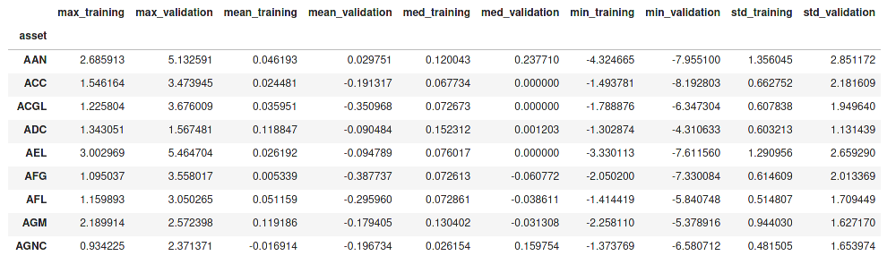
Example of a simple Pandas table with “assets” as index and various numerical columns
Similar to a table in a database, each DataFrame also has an index with unique keys to efficiently access individual rows or whole ranges of rows. The named columns of Pandas DataFrames can also be seen as a horizontal index which again allows you to efficiently access individual columns or ranges of columns.
Both the vertical row index and the horizontal column index can also contain multiple levels, which can be quite useful, for example for modelling stock prices of multiple different assets over time:
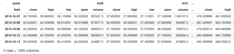
Example of nested column indices and a date as row index
Pandas provides a very orthogonal design with respect to rows and columns, they are interchangeable in most (but not all) functions. And if that is not possible, you can easily transpose a DataFrame, i.e. rotate the table by 90 degree to turn all rows into columns and vice versa. Note that this operation is something which is not possible with a traditional database.
Flexibility of Pandas
The Pandas DataFrame API is very flexible and providing more functionality than you’d find in SELECT statements in a traditional database. Let us have a quick look at the most basic ones, just to get a feeling and to be able to compare the functionality with Spark in the next part of this series.
For the following tiny examples, assume that we use a DataFrame persons with the following contents:

A Pandas DataFrame containing some persons
Since most (but not all) operations can also be performed in a traditional database, I will also mention the corresponding operation to put them into the perspective of a relational algebra.
Projections
One of the possibly simplest transformations is a projection, which simply creates a new DataFrame with a subset of the existing columns. This operation is called projection, because it is similar to a mathematical projection of a higher-dimensional space into a lower dimensional space (for example 3d to 2d). Specifically a projection reduces the number of dimensions and it is idempotent, i.e. performing the same projection a second time on the result will not change the data any more.

Projection of the persons DataFrame to the “age” and “height” column
A projection in SQL would be a very simple SELECT statement with a subset of all available columns.
Filtering
The next simple transformation in filtering, which only selects a subset of the available rows. It is similar to a projection, but works on rows instead of columns.

Filtering people, which are older than 21 years.
Filtering in SQL is typically performed within the WHERE clause.
Joins
Joins are an elementary operation in a relation database — without them, the term relational wouldn’t be very meaningful. Pandas joins require that the right DataFrame already is indexed by the join column.
For a small demonstration, I first load a second DataFrame containing the name of the city some persons live in:

Now we need to create an appropriate index for that DataFrame, otherwise Pandas refuses to perform the join operation:

Finally we can now perform the join operation:
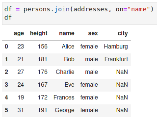
Note that this example shows that the term index really is appropriate as it provides a fast lookup mechanism, which is required for the join operation.
In SQL a join operation is performed via the JOIN clause as part of a SELECT statement.
#spark #pandas #python #data-science #developer