A Complete Guide To Time Series Forecasting

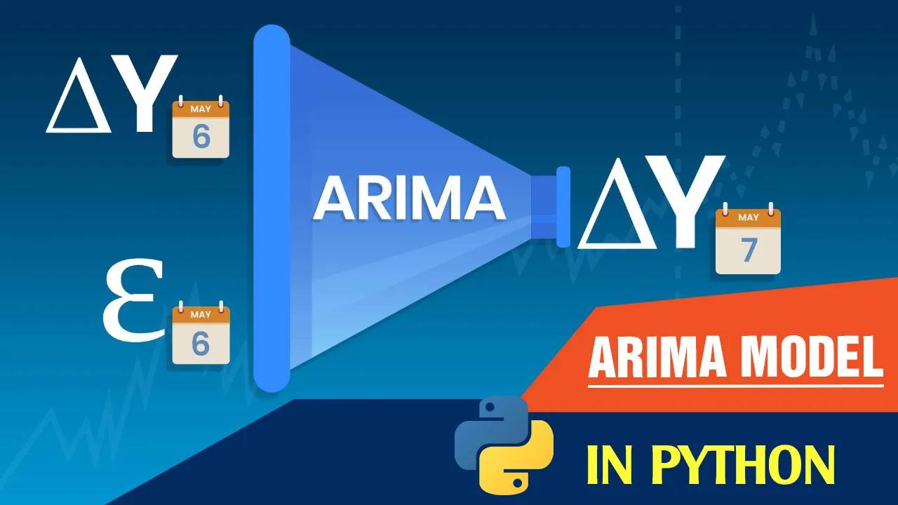
ARIMA is one of the most popular statistical models. It stands for AutoRegressive Integrated Moving Average and it’s fitted to time series data either for forecasting or to better understand the data. We will not cover the whole theory behind the ARIMA model but we will show you what’s the steps you need to follow to apply it correctly.

The key aspects of the ARIMA model are the following:

• AR: Autoregression. This indicates that the time series is regressed on its own lagged values.
• I: Integrated. This indicates that the data values have been replaced with the difference between their values and the previous values in order to convert the series into stationary.
• **MA: Moving Average. **This indicates that the regression error is actually a linear combination of error terms whose values occurred contemporaneously and at various times in the past.

The ARIMA model can be applied when we have seasonal or non-seasonal data. The difference is that when we have seasonal data we need to add some more parameters to the model.

For non-seasonal data the parameters are:

• p: The number of lag observations the model will use
• d: The number of times that the raw observations are differenced till stationarity.
• q: The size of the moving average window.

For seasonal data we need to add also the following:

• P: The number of seasonal lag observations the model will use
• D: The number of times that the seasonal observations are differenced till stationarity.
• Q: The size of the seasonal moving average window.
• m: The number of observations of 1 season

#forecasting #data-science #arima #timeseries #python