In the first article of this three-part series, we saw the basics of the Kaplan-Meier Estimator. Now, it’s time to implement the theory we discussed in the first part.
Example 1: Kaplan-Meier Estimator (Without any groups)
Let’s code:
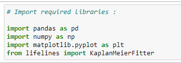
(1) Import required libraries:
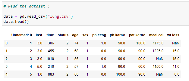
(2) Read the dataset:
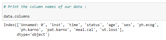
(3) Columns of our dataset:
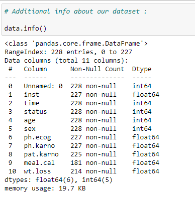
(4) Additional info about dataset:
It gives us information about the data types and the number of rows in each column that has null values. It’s very important for us to remove the rows with a null value for some of the methods in survival analysis.
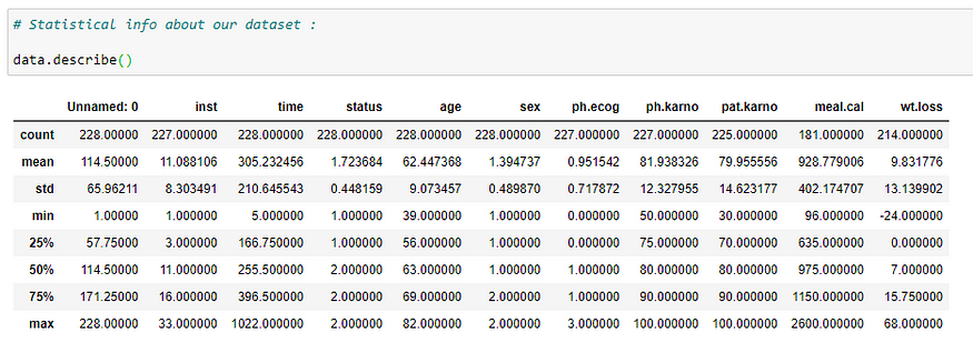
(5) Statistical info about dataset:
It gives us some statistical information like the total number of rows, mean, standard deviation, minimum value, 25th percentile, 50th percentile, 75th percentile, and maximum value for each column in our dataset.
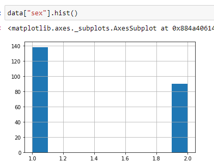
(6) Find out sex distribution using histogram:
This gives us a general idea about how our data is distributed. In the following graph, you can see that around 139 values have a status of 1, and around 90 values have a status of 2. It means that in our dataset, there are 139 males and around 90 females.
(7) Create an object for KaplanMeierFitter:
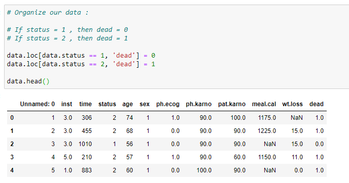
(8) Organize the data:
Now we need to organize our data. We’ll add a new column in our dataset that is called “dead”. It stores the data about whether a person that is a part of our experiment is dead or alive (based on the status value). If our status value is 1 then that person is alive, and if our status value is 2 then the person is dead. It’s a very crucial step for what we need to do in the next step. As we are going to store our data in columns called censored and observed. Where observed data stores the value of dead persons in a specific timeline and censored data stores the value of alive persons or persons that we’re not going to investigate at that timeline.
(9) Fitting our data into object:
Here our goal is to find the number of days a patient survived before they died. So our event of interest will be “death”, which is stored in the “dead” column. The first argument it takes is the timeline for our experiment.
#2020 jul tutorials #overviews #python #statistics #survival analysis #data analysis