Step-by-Step Guide to Creating R and Python Libraries (in JupyterLab)

Using Docker and JupyterLab to create R and Python Libraries.

R and Python are the bread and butter of today’s machine learning languages. R provides powerful statistics and quick visualizations, while Python offers an intuitive syntax, abundant support, and is the choice interface to today’s major AI frameworks.

In this article we’ll look at the steps involved in creating libraries in R and Python. This is a skill every machine learning practitioner should have in their toolbox. Libraries help us organize our code and share it with others, offering packaged functionality to the data community.

Building today’s software doesn’t happen without extensive use of libraries. Libraries dramatically cut down the time and effort required for a team to bring work to production. By leveraging the open source community engineers and scientists can move their unique contribution towards a larger audience, and effectively improve the quality of their code. Companies of all sizes use these libraries to sit their work on top of existing functionality, making product development more productive and focused.

But creating libraries isn’t just for production software. Libraries are critical to rapidly prototyping ideas, helping teams validate hypotheses and craft experimental software quickly. While popular libraries enjoy massive community support and a set of best practices, smaller projects can be converted into libraries overnight.

By learning to create lighter-weight libraries we develop an ongoing habit of maintaining code and sharing our work. Our own development is sped up dramatically, and we anchor our coding efforts around a tangible unit of work we can improve over time.

ARTICLE SCOPE

In this article we will focus on creating libraries in R and Python as well as hosting them on, and installing from, GitHub. This means we won’t look at popular hosting sites like CRAN for R and PyPI for Python. These are extra steps that are beyond the scope of this article.

Focusing only on GitHub helps encourage practitioners to develop and share libraries more frequently. CRAN and PyPI have a number of criteria that must be met (and they change frequently), which can slow down the process of releasing our work. Rest assured, it is just as easy for others to install our libraries from GitHub. Also, the steps for CRAN and PyPI can always be added later should you feel your library would benefit from a hosting site.

We will build both R and Python libraries using the same environment (JupyterLab), with the same high-level steps for both languages. This should help you build a working knowledge of the core step required to package your code as a library.

Let’s get started.

SETUP

We will be creating a library called datapeek in both R and Python. The datapeek library is a simple package offering a few useful functions for handling raw data. These functions are:

encode_and_bind

remove_features

apply_function_to_column

get_closest_string

We will look at these functions later. For now we need to setup an R and Python environment to create datapeek, along with a few libraries to support packaging our code. We will be using JupyterLab inside a Docker container, along with a “docker stack” that comes with the pieces we need.

Install and Run Docker

The Docker Stack we will use is called the jupyter/datascience-notebook. This image contains both R and Python environments, along with many of the packages typically used in machine learning.

Since these run inside Docker you must have Docker installed on your machine. So install Docker if you don’t already have it, and once installed, run the following in terminal to pull the datascience-notebook:

docker pull jupyter/datascience-notebook

This will pull the most recent image hosted on Docker Hub.

Once everything has been pulled we can confirm our new image exists by running the following:

docker images

… showing something similar to the following:

Now that we have our Docker stack let’s setup JupyterLab.

JupyterLab

We will create our libraries inside a JupyterLab environment. JupyterLab is a web-based user interface for programming. With JupyterLab we have a lightweight IDE in the browser, making it convenient for building quick applications. JupyterLab provides everything we need to create libraries in R and Python, including:

A terminal environment for running shell commands and downloading/installing libraries;
An R and Python console for working interactively with these languages;
A simple text editor for creating files with various extensions;
Jupyter Notebooks for prototyping ML work.

The datascience-notebook we just pulled contains an installation of JupyterLab so we don’t need to install this separately. Before running our Docker image we need to mount a volume to ensure our work is saved outside the container.

First, create a folder called datapeek on your desktop (or anywhere you wish) and change into that directory. We need to run our Docker container with JupyterLab,so our full command should look as follows:

docker run -it -v `pwd`:/home/jovyan/work -p 8888:8888 jupyter/datascience-notebook start.sh jupyter lab

You can learn more about Docker commands here. Importantly, the above command exposes our environment on port 8888, meaning we can access our container through the browser.

After running the above command you should see the following output at the end:

This tells us to copy and paste the provided URL into our browser. Open your browser and add the link in the address bar and hit enter (your token will be different):

localhost:8888/?token=11e5027e9f7cacebac465d79c9548978b03aaf53131ce5fd

This will automatically open JupyterLab in your browser as a new tab:

We are now ready to start building libraries.

We begin this article with R, then look at Python.

CREATING LIBRARIES IN R

R is one of the “big 2” languages of machine learning. At the time of this writing it has well-over 10,000 libraries. Going toAvailable CRAN Packages By Date of Publication and running…

document.getElementsByTagName('tr').length

…in the browser console gives me 13858. Minus the header and final row this gives 13856 packages. Needless to say R is not in need of variety. With strong community support and a concise (if not intuitive) language, R sits comfortably at the top of statistical languages worth learning.

The most well-known treatise on creating R packages is Hadley Wickam’s book R Packages. Its contents are available for free online. For a deeper dive on topic I recommend looking there.

We will use Hadley’s devtools package to abstract away the tedious tasks involved in creating packages. devtools is already installed in our Docker Stacks environment. We also require the roxygen2 package, which helps us document our functions. Since this doesn’t come pre-installed with our image let’s install that now.

Inside the console type R, then….

install.packages("roxygen2")
library("roxygen2")

With the necessary packages installed we’re ready to tackle each step.

STEP 1: Create Package Framework

We need to create a directory for our package. We can do this in one line of code, using the devtools create function. In terminal run:

devtools::create("datapeek")

This automatically creates the bare bone files and directories needed to define our R package. In JupyterLab you will see a set of new folders and files created on the left side.

datapeek
├── R
├── datapeek.Rproj
├── DESCRIPTION
├── NAMESPACE

The R folder will eventually contain our R code. The my_package.Rproj file is specific to the RStudio IDE so we can ignore that. The DESCRIPTION folder holds our package’s metadata (adetailed discussion can be found here). Finally, NAMSPACE is a file that ensures our library plays nicely with others, and is more of a CRAN requirement.

Naming Conventions

We must follow these rules when naming an R package:

A terminal environment for running shell commands and downloading/installing libraries;
An R and Python console for working interactively with these languages;
A simple text editor for creating files with various extensions;
Jupyter Notebooks for prototyping ML work.

You can read more about naming packages here. Our package name “datapeek” passes the above criteria. Let’s head over to CRAN and do a Command+F search for “datapeek” to ensure it’s not already taken:

Command + F search on CRAN to check for package name uniqueness.

…look’s like we’re good.

STEP 2: Fill Out Description Details

The job of the DESCRIPTION file is to store important metadata about our package. These data include others packages required to run our library, our license, and our contact information. Technically, the definition of a package in R is any directory containing a DESCRIPTION file, so always ensure this is present.

Click on the DESCRIPTION file in JupyterLab’s directory listing. You will see the basic details created automatically when we ran devtools::create(“datapeek”) :

Let’s add our specific details so our package contains the necessary metadata. Simply edit this file inside JupyterLab. Here are the details I am adding:

A terminal environment for running shell commands and downloading/installing libraries;
An R and Python console for working interactively with these languages;
A simple text editor for creating files with various extensions;
Jupyter Notebooks for prototyping ML work.

Of course you should fill out these parts with your own details. You can read more about the definitions of each of these in Hadley’s chapter on metadata. As a brief overview…the package, title, and version parts are self-explanatory, just be sure to keep title to one line. Authors@R must adhere to the format you see above, since it contains executable R code. Note the role argument, which allows us to list the main contributors of our library. The usual ones are:

aut: author

cre: creator or maintainer

ctb: contributors

cph: copyright holder

There are many more options, with the full list found here.

You can add multiple authors by listing them as a vector:

Authors@R: as.person(c(
    "Sean McClure <sean.mcclure@example.com> [aut, cre]", 
    "Rick Deckard <rick.deckard@example.com> [aut]",
    "Rachael Tyrell <rachel.tyrell@example.com> [ctb]"
))

STEP 3: Add Functions

3A: Add Functions to R Folder

Our library wouldn’t do much without functions. Let’s add the 4 functions mentioned in the beginning of this article. The following GIST shows our datapeek functions in R:

library(data.table)
library(mltools)

encode_and_bind <- function(frame, feature_to_encode) {
    res <- cbind(iris, one_hot(as.data.table(frame[[feature_to_encode]])))
    return(res)
}

remove_features <- function(frame, features) {
  rem_vec <- unlist(strsplit(features, ', '))
  res <- frame[,!(names(frame) %in% rem_vec)]
  return(res)
}

apply_function_to_column <- function(frame, list_of_columns, new_col, funct) {
    use_cols <- unlist(strsplit(list_of_columns, ', '))
    new_cols <- unlist(strsplit(new_col, ', '))
    frame[new_cols] <- apply(frame[use_cols], 2, function(x) {eval(parse(text=funct))})
    return(frame)
}

get_closest_string <- function(vector_of_strings, search_string) {
    all_dists <- adist(vector_of_strings, search_string)
    closest <- min(all_dists)
    res <- vector_of_strings[which(all_dists == closest)]
    return(res)
}

We have to add our functions to the R folder, since this is where R looks for any functions inside a library.

datapeek
├── R
├── datapeek.Rproj
├── DESCRIPTION
├── NAMESPACE

Since our library only contains 4 functions we will place all of them into a single file called utilities.R, with this file residing inside the R folder.

Go into the directory in JupyterLab and open the R folder. Click on Text File in the Launcher and paste in our 4 R functions. Right-click the file and rename it to utilities.R.

3B: Export our Functions

It isn’t enough to simply place R functions in our file. Each function must be exported to expose them to users of our library. This is accomplished by adding the @export tag above each function.

The export syntax comes from Roxygen, and ensures our function gets added to the NAMESPACE. Let’s add the @export tag to our first function:

#' @export
encode_and_bind <- function(frame, feature_to_encode) {
    res <- cbind(iris, one_hot(as.data.table(frame[[feature_to_encode]])))
    return(res)
}

Do this for the remaining functions as well.

It is important to document our functions. Documenting functions provides information for users, such that when they type ?datapeek they get details about our package. Documenting also supports working with vignettes, which are a long-form type of documentation. You can read more about documenting functions here.

There are 2 sub-steps we will take:

A terminal environment for running shell commands and downloading/installing libraries;
An R and Python console for working interactively with these languages;
A simple text editor for creating files with various extensions;
Jupyter Notebooks for prototyping ML work.

— Add the Document Annotations

Documentation is added above our function, directly above our #’ @export line. Here’s the example with our first function:

#' One-hot encode categorical variables.
#'
#' This function one-hot encodes categorical variables and binds the entire frame.
#'
#' @param data frame
#' @param feature to encode
#' @return hot-encoded data frame
#'
#' @export
encode_and_bind <- function(frame, feature_to_encode) {
    res <- cbind(iris, one_hot(as.data.table(frame[[feature_to_encode]])))
    return(res)
}

We space out the lines for readability, adding a title, description, and any parameters used by the function. Let’s do this for our remaining functions:

library(data.table)
library(mltools)

#' One-hot encode categorical variables.
#'
#' This function one-hot encodes categorical variables and binds the entire frame.
#'
#' @param data frame
#' @param feature to encode
#' @return hot-encoded data frame
#'
#' @export
encode_and_bind <- function(frame, feature_to_encode) {
    res <- cbind(iris, one_hot(as.data.table(frame[[feature_to_encode]])))
    return(res)
}

#' Remove specified features from data frame.
#'
#' This function removes specified features from data frame.
#'
#' @param data frame
#' @param features to remove
#' @return original data frame less removed features
#'
#' @export
remove_features <- function(frame, features) {
  rem_vec <- unlist(strsplit(features, ', '))
  res <- frame[,!(names(frame) %in% rem_vec)]
  return(res)
}

#' Apply function to multiple columns.
#'
#' This function enables the application of a function to multiple columns.
#'
#' @param data frame
#' @param list of columns to apply function to
#' @param name of new column
#' @param function to apply
#' @return original data frame with new column attached 
#'
#' @export
apply_function_to_column <- function(frame, list_of_columns, new_col, funct) {
    use_cols <- unlist(strsplit(list_of_columns, ', '))
    new_cols <- unlist(strsplit(new_col, ', '))
    frame[new_cols] <- apply(frame[use_cols], 2, function(x) {eval(parse(text=funct))})
    return(frame)
}

#' Discover closest matching string from set.
#'
#' This function discovers the closest matching string from vector of strings.
#'
#' @param vector of strings
#' @param search string
#' @return closest matching string
#'
#' @export
get_closest_string <- function(vector_of_strings, search_string) {
    all_dists <- adist(vector_of_strings, search_string)
    closest <- min(all_dists)
    res <- vector_of_strings[which(all_dists == closest)]
    return(res)
}

— Run devtools::document()

With documentation added to our functions we then run the following in terminal,just outside the root directory:

devtools::document()

Error: ‘roxygen2’ >= 5.0.0 must be installed for this functionality.

In this case open terminal in JupyterLab and install roxygen2. You should also install data.table and mltools, since our first function uses these:

install.packages('roxygen2')
install.packages('data.table')
install.packages('mltools')

Run the devtools::document() again. You should see the following:

This will generate .Rd files inside a new man folder. You’ll notice an .Rd file is created for each function in our package.

If you look at your DESCRIPTION file it will now show a new line at the bottom:

This will also generate a NAMESPACE file:

We can see our 4 functions have been exposed. Let’s now move onto ensuring dependencies are specified inside our library.

STEP 4: List External Dependencies

It is common for our functions to require functions found in other libraries. There are 2 things we must do to ensure external functionality is made available to our library’s functions:

Use double colons inside our functions to specify which library we are relying on;
Add imports to our DESCRIPTION file.

You’ll notice in the above GIST we simply listed our libraries at the top. While this works well in stand-alone R scripts it isn’t the way to use dependencies in an R package. When creating R packages we must use the “double-colon approach” to ensure the correct function is read. This is related to how “top-level code” (code that isn’t an object like a function) in an R package is only executed when the package is built, not when it’s loaded.

For example:

library(mltools)

do_something_cool_with_mltools <- function() {
    auc_roc(preds, actuals)
}

…won’t work because auc_roc will not be available (running library(datapeek) doesn’t re-execute library(mltools)). This will work:

do_something_cool_with_mltools <- function() {
    mltools::auc_roc(preds, actuals)
}

The only function in our datapeek package requiring additional packages is our first one:

#' One-hot encode categorical variables.
#'
#' This function one-hot encodes categorical variables and binds the entire frame.
#'
#' @param data frame
#' @param feature to encode
#' @return hot-encoded data frame
#'
#' @export
encode_and_bind <- function(frame, feature_to_encode) {
    res <- cbind(iris, mltools::one_hot(data.table::as.data.table(frame[[feature_to_encode]])))
    return(res)
}

Using the double-colon approach to specify dependent packages in R.

Notice each time we call an external function we preface it with the external library and double colons.

We must also list external dependencies in our DESCRIPTION file, so they are handled correctly. Let’s add our imports to the DESCRIPTION file:

Be sure to have the imported libraries comma-separated. Notice we didn’t specify any versions for our external dependencies. If we need to specify versions we can use parentheses after the package name:

Imports:
    data.table (>= 1.12.0)

Since our encode_and_bind function isn’t taking advantage of any bleeding-edge updates we will leave it without any version specified.

STEP 5: Add Data

Sometimes it makes sense to include data inside our library. Package data can allow our user’s to practice with our library’s functions, and also helps with testing, since machine learning packages will always contain functions that ingest and transform data. The 4 options for adding external data to an R package are:

Use double colons inside our functions to specify which library we are relying on;
Add imports to our DESCRIPTION file.

You can learn more about these different approaches here. For this article we will stick with the most common approach, which is to add external data to an R folder.

Let’s add the Iris dataset to our library in order to provide users a quick way to test our functions. The data must be in the .rda format, created using R’s **save()** function, and have the same name as the file. We can ensure these criteria are satisfied by using devtools’ use_data function:

x <- read.csv("http://bit.ly/2HuTS0Z")
devtools::use_data(x, iris)

Above, I read in the Iris dataset from its URL and pass the data frame to devtools::use_data().

In JupyterLab we see a new data folder has been created, along with our iris.rda dataset:

datapeek
├── data
    └── iris.rda
├── man
├── R
├── datapeek.Rproj
├── DESCRIPTION
├── NAMESPACE

We will use our added dataset to run tests in the following section.

STEP 6: Add Tests

Testing is an important part of software development. Testing helps ensure our code works as expected, and makes debugging our code a much faster and more effective process. Learn more about testing R packages here.

A common challenge in testing is knowing what we should test. Testing every function in a large library is cumbersome and not always needed, while not enough testing can make it harder to find and correct bugs when they arise.

I like the following quote from Martin Fowler regarding when to test:

The interactive testing we do in data science is manual, but what we are looking for in our packages is automated testing. Automated testing means we run a suite of pre-defined tests to ensure our package works end-to-end.

While there are many kinds of tests in software, here we are taking about “unit tests.” Thinking in terms of unit tests forces us to break up our code into more modular components, which is good practice in software design.

6A: Creating the tests/testthat folder;

6B: Writing tests.

— 6A: Creating the **tests/testthat** folder

Just as R expects our R scripts and data to be in specific folders it also expects the same for our tests. To create the tests folder, we run the following in JupyterLab’s R console:

devtools::use_testthat()

You may get the following error:

Error: ‘testthat’ >= 1.0.2 must be installed for this functionality.

If so, use the same approach above for installing roxygen2 in Jupyter’s terminal.

install.packages('testthat')

Running devtools::use_testthat() will produce the following output:

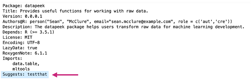
* Adding testthat to Suggests
* Creating `tests/testthat`.
* Creating `tests/testthat.R` from template.

There will now be a new tests folder in our main directory:

datapeek
├── data
├── man
├── R
├── tests
    └── testthat.R
├── datapeek.Rproj
├── DESCRIPTION
├── NAMESPACE

The above command also created a file called testthat.R inside the tests folder. This runs all your tests when R CMD check runs (we’ll look at that shortly). You’ll also notice_testthat_ has been added under Suggests in our DESCRIPTION file:

— 6B: Writing Tests

testthat is the most popular unit testing package for R, used by at least 2,600 CRAN package, not to mention libraries on Github. You can check out the latest news regarding testthat on the Tidyverse page here. Also check out its documentation.

There are 3 levels to testing we need to consider:

A terminal environment for running shell commands and downloading/installing libraries;
An R and Python console for working interactively with these languages;
A simple text editor for creating files with various extensions;
Jupyter Notebooks for prototyping ML work.

Assertions

Assertions are the functions included in the testing library we choose. We use assertions to check whether our own functions return the expected output. Assertions come in many flavors, depending on what is being checked. In the following section I will cover the main tests used in R programming, showing each one failing so you can understand how it works.

Equality Assertions

A terminal environment for running shell commands and downloading/installing libraries;
An R and Python console for working interactively with these languages;
A simple text editor for creating files with various extensions;
Jupyter Notebooks for prototyping ML work.

# test for equality
a <- 10
expect_equal(a, 14)

> Error: `a` not equal to 14.

# test for identical 
expect_identical(42, 2)

> Error: 42 not identical to 2.

# test for equivalence 
expect_equivalent(10, 12)

> Error: 10 not equivalent to 12.

There are subtle differences between the examples above. For example, expect_equal is used to check for equality within a numerical tolerance, while expect_identical tests for exact equivalence. Here are examples:

expect_equal(10, 10 + 1e-7) # true
expect_identical(10, 10 + 1e-7) # false

As you write more tests you’ll understand when to use each one. Of course always refer to the documentation referenced above when in doubt.

Testing for String Matches

A terminal environment for running shell commands and downloading/installing libraries;
An R and Python console for working interactively with these languages;
A simple text editor for creating files with various extensions;
Jupyter Notebooks for prototyping ML work.

# test for string matching
expect_match("Machine Learning is Fun", "But also rewarding.")

> Error: "Machine Learning is Fun" does not match "But also rewarding.".

Testing for Length

A terminal environment for running shell commands and downloading/installing libraries;
An R and Python console for working interactively with these languages;
A simple text editor for creating files with various extensions;
Jupyter Notebooks for prototyping ML work.

# test for length 
vec <- 1:10
expect_length(vec, 12)

> Error: `vec` has length 10, not length 12.

Testing for Comparison

A terminal environment for running shell commands and downloading/installing libraries;
An R and Python console for working interactively with these languages;
A simple text editor for creating files with various extensions;
Jupyter Notebooks for prototyping ML work.

# test for less than
a <- 11
expect_lt(a, 10)

> Error: `a` is not strictly less than 10. Difference: 1

# test for greater than
a <- 11
expect_gt(a, 12)

> Error: `a` is not strictly more than 12. Difference: -1

Testing for Logic

A terminal environment for running shell commands and downloading/installing libraries;
An R and Python console for working interactively with these languages;
A simple text editor for creating files with various extensions;
Jupyter Notebooks for prototyping ML work.

# test for truth 
expect_true(5 == 2)

> Error: 5 == 2 isn't true.

# test for false 
expect_false(2 == 2)

> Error: 2 == 2 isn't false.

Testing for Outputs

A terminal environment for running shell commands and downloading/installing libraries;
An R and Python console for working interactively with these languages;
A simple text editor for creating files with various extensions;
Jupyter Notebooks for prototyping ML work.

# testing for outputs 
expect_output(str(mtcars), "31 obs")

> Error: `str\(mtcars\)` does not match "31 obs".

# test for warning 
f <-function(x) {
  if(x < 0) {
    message("*x* is already negative")
  }
}

expect_message(f(1))

> Error: `f(1)` did not produce any messages.

There are many more included in the testthat library. If you are new to testing, start writing a few simple ones to get used to the process. With time you’ll build an intuition around what to test and when.

Writing Tests

A test is a group of assertions. We write tests in testthat as follows:

test_that("this functionality does what it should", {
    // group of assertions here
})

We can see we have both a description (the test name) and the code (containing the assertions). The description completes the sentence, “test that ….”

Above, we are saying “test that this functionality does what it should.”

The assertions are the outputs we wish to test. For example:

test_that("trigonometric functions match identities", {
      expect_equal(sin(pi / 4), 1 / sqrt(2))
      expect_equal(cos(pi / 4), 1 / sqrt(10))
      expect_equal(tan(pi / 4), 1)
    })

> Error: Test failed: 'trigonometric functions match identities'

The last thing we do in testing is create files. As stated above, a“file” in testing is a group of tests covering a related set of functionality. Our test file must live inside thetests/testthat/ directory. Here is an example test file for the stringr package on GitHub:

Example Test File from the stringr package on GitHub.

The file is called test-case.R (starts with “test”) and lives inside the tests/testthat/ directory. The context at the top simply allows us to provide a simple description of the file’s contents. This appears in the console when we run our tests.

Let’s create our test file, which will contain tests and assertions related to our 4 functions. As usual, we use JupyterLab’s Text File in Launcher to create and rename a new file:

Creating a Test File in R

Now let’s add our tests:

For the first function I am going to make sure a data frame with the correct number of features is returned:

context('utility functions')

library(data.table)
library(mltools)

load('../../data/iris.rda')

test_that("data frame with correct number of features is returned", {
    res <- encode_and_bind(iris, 'Species')
    expect_equal(dim(res)[2], 8)
})

Notice how we called our encode_and_bind function, then simply checked the equality between the dimensions and the expected output. We run our automated tests at any point to ensure our test file runs and we get the expected output. Running devtools::test() in the console runs our tests:

We get a smiley face too!

Since our second function removes a specified feature I will use the same test as above, checking for the dimensions of the returned frame. Our third function applies a specified function to a chosen column, so I will write a test that checks the result of given specified function. Finally, our fourth function returns the closest matching string, so I will simply check the returned string for the expected result.

Here is our full test file:

context('utility functions')

library(data.table)
library(mltools)

load('../../data/iris.rda')

test_that("data frame with correct number of features is returned", {
    res <- encode_and_bind(iris, 'Species')
    expect_equal(dim(res)[2], 8)
})

test_that("data frame with correct number of features is returned", {
    res <- remove_features(iris, 'Species')
    expect_equal(dim(res)[2], 4)
})

test_that("newly created columns return correct sum", {
    res <- apply_function_to_column(iris, "Sepal.Width, Sepal.Length", "new_col1, new_col2", "x*5") 
    expect_equal(sum(res$new_col1), 2293)
    expect_equal(sum(res$new_col2), 4382.5)
})

test_that("closest matching string is returned", {
    res <- get_closest_string(c("hey there", "we are here", "howdy doody"), "doody") 
    expect_true(identical(res, 'howdy doody'))
})

As we did above, we run our tests using the following command:

devtools::test()

This will run all tests in any test files we placed inside the testthat directory. Let’s check the result:

We had 5 assertions across 4 unit tests, placed in one test file. Looks like we’re good. If any of our tests failed we would see this in the above printout, at which point we would look to correct the issue.

STEP 7: Create Documentation

This has traditionally been done using “Vignettes” in R. You can learn about creating R vignettes for your R package here. Personally, I find this a dated approach to documentation. I prefer to use things like Sphinx or Julep. Documentation should be easily shared, searchable and hosted.

Click on the question mark at julepcode.com to learn how to use Julep.

I created and hosted some simple documentation for our R datapeek library, which you can find here.

Of course we will also have the library on GitHub, which I cover below.

STEP 8: Share your R Library

As I mentioned in the introduction we should be creating libraries on a regular basis, so others can benefit from and extend our work. The best way to do this is through GitHub, which is the standard way to distribute and collaborate on open source software projects.

In case you’re new to GitHub here’s a quick tutorial to get you started so we can push our datapeek project to a remote repo.

…which will provide us with the usual screen:

With our remote repo setup we can initialize our local repo on our machine, and send our first commit.

Open Terminal in JupyterLab and change into the datapeek directory:

Initialize the local repo:

git init

Add the remote origin (your link will be different):

git remote add origin https://github.com/sean-mcclure/datapeek.git

Now run git add . to add all modified and new (untracked) files in the current directory and all subdirectories to the staging area:

git add .

Don’t forget the “dot” in the above command. Now we can commit our changes, which adds any new code to our local repo.

But, since we are working inside a Docker container the username and email associated with our local repo cannot be autodetected. We can set these by running the following in terminal:

git config --global user.email {emailaddress}
git config --global user.name {name}

Use the email address and username you use to sign into GitHub.

Now we can commit:

git commit -m 'initial commit'

With our new code committed we can do our push, which transfers the last commit(s) to our remote repo:

git push origin master

### R ###
# History files
.Rhistory
.Rapp.history

# Session Data files
.RData

# User-specific files
.Ruserdata

# Example code in package build process
*-Ex.R

# Output files from R CMD build
/*.tar.gz

# Output files from R CMD check
/*.Rcheck/

# RStudio files
.Rproj.user/

# produced vignettes
vignettes/*.html
vignettes/*.pdf

# OAuth2 token, see https://github.com/hadley/httr/releases/tag/v0.3
.httr-oauth

# knitr and R markdown default cache directories
/*_cache/
/cache/

# Temporary files created by R markdown
*.utf8.md
*.knit.md

### R.Bookdown Stack ###
# R package: bookdown caching files
/*_files/

Example .gitignore file for an R package

To recap, git add adds all modified and new (untracked) files in the current directory to the staging area. Commit adds any changes to our local repo, and push transfers the last commit(s) to our remote repo. While git add might seem superfluous, the reason it exists is because sometimes we want to only commit certain files, this we can stage files selectively. Above, we staged all files by using the “dot” after git add.

You may also notice we didn’t include a README file. You should indeed include this, however for the sake of brevity I have left this step out.

Now, anyone can use our library. 👍 Let’s see how.

STEP 9: Install your R Library

As mentioned in the introduction I will not be discussing CRAN in this article. Sticking with GitHub make it easier to share our code frequently, and we can always add CRAN criteria later.

To install a library from GitHub, users can simply run the following command on their local machine:

devtools::install_github("yourusername/mypackage")

As such, we can simply instruct others wishing to use datapeek to run the following command on their local machine:

devtools::install_github("sean-mcclure/datapeek")

This is something we would include in a README file and/or any other documentation we create. This will install our package like any other package we get from CRAN:

Users then load the library as usual and they’re good to go:

library(datapeek)

I recommend trying the above commands in a new R environment to confirm the installation and loading of your new library works as expected.

CREATING LIBRARIES IN PYTHON

Creating Python libraries follows the same high-level steps we saw previously for R. We require a basic directory structure with proper naming conventions, functions with descriptions, imports, specified dependencies, added datasets, documentation, and the ability to share and allow others to install our library.

We will use JupyterLab to build our Python library, just as we did for R.

Library vs Package vs Module

In the beginning of this article I discussed the difference between a “library” and a “package”, and how I prefer to use these terms interchangeably. The same holds for Python libraries. “Modules” are another term, and in Python simply refer to any file containing Python code. Python libraries obviously contain modules as scripts.

Before we start:

I stated in the introduction that we will host and install our libraries on and from GitHub. This encourages rapid creation and sharing of libraries without getting bogged down by publishing criteria on popular package hosting sites for R and Python.

The most popular hosting site for Python is the Python Package Index (PyPI). This is a place for finding, installing and publishing python libraries. Whenever you run pip install <package_name> (or easy_intall) you are fetching a package from PyPI.

While we won’t cover hosting our package on PyPI it’s still a good idea to see if our library name is unique. This will minimize confusion with other popular Python libraries and improve the odds our library name is distinctive, should we decide to someday host it on PyPI.

First, we should follow a few naming conventions for Python libraries.

Python Library Naming Conventions

A terminal environment for running shell commands and downloading/installing libraries;
An R and Python console for working interactively with these languages;
A simple text editor for creating files with various extensions;
Jupyter Notebooks for prototyping ML work.

Our library name is datapeek, so the first and third criteria are met; let’s check PyPI for uniqueness:

All good. 👍

We’re now ready to move through each step required to create a Python library.

STEP 1: Create Package Framework

JupyterLab should be up-and-running as per the instructions in the setup section of this article.

Use JupyterLab’s New Folder and Text File options to create the following directory structure and files:

datapeek
├── datapeek
    └── __init__.py
    └── utilities.py
├── setup.py

There will be files we do not want to commit to source control. These are files that are created by the Python build system. As such, let’s alsoadd the following** .gitignore file** to our package framework:

# Compiled python modules.
*.pyc

# Setuptools distribution folder.
/dist/

# Python egg metadata, regenerated from source files by setuptools.
/*.egg-info

datapeek
├── datapeek
    └── __init__.py
    └── utilities.py
├── setup.py
├── gitignore

STEP 2: Fill Out Description Details

Just as we did for R, we should add metadata about our new library. We do this using Setuptools. Setuptools is a Python library designed to facilitate packaging Python projects.

**Open **setup.py and add the following details for our library:

from setuptools import setup

setup(name='datapeek',
      version='0.1',
      description='A simple library for dealing with raw data.',
      url='https://github.com/sean-mcclure/datapeek_py',
      author='Sean McClure',
      author_email='sean.mcclure@example.com',
      license='MIT',
      packages=['datapeek'],
zip_safe=False)

Of course you should change the authoring to your own. We will add more details to this file later. The keywords are fairly self-explanatory. url is the URL of our project on GitHub, which we will add later; unless you’ve already created your python repo, in which case add the URL now. We talked about licensing in the R section. zip_safe simply means our package can be run safely as a zip file which will usually be the case. You can learn more about what can be added to the setup.py file here.

STEP 3: Add Functions

Our library obviously requires functions to be useful. For larger libraries we would organize our modules so as to balance cohesion/coupling, but since our library is small we will simply keep all functions inside a single file.

We will add the same functions we did for R, this time written in Python:

import pandas as pd
from fuzzywuzzy import fuzz

def encode_and_bind(frame, feature_to_encode):
    dummies = pd.get_dummies(frame[[feature_to_encode]])
    res = pd.concat([frame, dummies], axis=1)
    res = res.drop([feature_to_encode], axis=1)
    return(res)

def remove_features(frame, list_of_columns):
    res = frame.drop(frame[list_of_columns],axis=1)
    return(res)

def apply_function_to_column(frame, list_of_columns, new_col, funct):
    frame[new_col] = frame[list_of_columns].apply(lambda x: eval(funct))
    return(frame)

def get_closest_string(list_of_strings, search_string):
    all_dists = []
    all_strings = []
    for string in list_of_strings:
        dist = fuzz.partial_ratio(string, search_string)
        all_dists.append(dist)
        all_strings.append(string)
    top = max(all_dists)
    ind=0
    for i, x in enumerate(all_dists):
        if x == top:
            ind = i
return(all_strings[ind])

Add these functions to the utilities.py module, inside datapeek’s module directory.

STEP 4: List External Dependencies

Our library will often require other packages as dependencies. Our user’s Python environment will need to be aware of these when installing our library (so these other packages can also be installed). Setuptools provides the install_requires keyword to list any packages our library depends on.

Our datapeek library depends on the fuzzywuzzy package for fuzzy string matching, and the pandas package for high-performance manipulation of data structures. To specify our dependencies**,** add the following to your setup.py file:

install_requires=[
    'fuzzywuzzy',
    'pandas'
]

Your setup.py file should currently look as follows:

from setuptools import setup

setup(name='datapeek',
      version='0.1',
      description='A simple library for dealing with raw data.',
      url='https://github.com/sean-mcclure/datapeek_py',
      author='Sean McClure',
      author_email='sean.mcclure@example.com',
      license='MIT',
      packages=['datapeek'],
      install_requires=[
          'fuzzywuzzy',
          'pandas'
      ],
zip_safe=False)

We can confirm all is in order by running the following in a JupyterLab terminal session:

python setup.py develop

…with an ending that reads:

Finished processing dependencies for datapeek==0.1

If one or more of our dependencies is not available on PyPI, but is available on GitHub (e.g. a bleeding-edge machine learning package is only available on Github…or it’s another one of our team’s libraries hosted only on GitHub), we can use dependency_links inside our setup call:

setup(
    ...
    dependency_links=['http://github.com/user/repo/tarball/master#egg=package-1.0'],
    ...
)

If you want to add additional metadata, such as status, licensing, language version, etc. we can use classifiers like this:

setup(
    ...
    classifiers=[
        'Development Status :: 3 - Alpha',
        'License :: OSI Approved :: MIT License',
        'Programming Language :: Python :: 2.7',
        'Topic :: Text Processing :: Linguistic',
      ],
    ...
)

To learn more about the different classifiers that can be added to our setup.py file see here.

STEP 5: Add Data

Just as we did above in R we can add data to our Python library. In Python these are called Non-Code Files and can include things like images, data, documentation, etc.

We add data to our library’s module directory, so that any code that requires those data can use a relative path from the consuming module’s __file__ variable.

Let’s add the Iris dataset to our library in order to provide users a quick way to test our functions. First, use the New Folder button in JupyterLab to create a new folder called data inside the module directory:

datapeek
├── datapeek
    └── __init__.py
    └── utilities.py
    └── data
├── setup.py
├── git

…then make a new Text File inside the data folder called iris.csv, and paste the data from here into the new file.

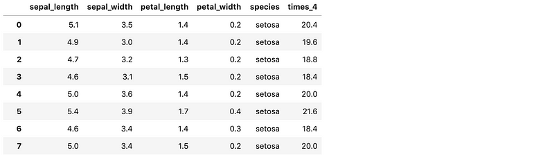
If you close and open the new csv file it will render inside JupyterLab as a proper table:

CSV file rendered in JupyterLab as formatted table.

We specify Non-Code Files using a MANIFEST.in file. Create another Text File called MANIFEST.in placing it inside your root folder:

datapeek
├── datapeek
    └── __init__.py
    └── utilities.py
    └── data
├── MANIFEST.in
├── setup.py
├── gitignore

…and add this line to the file:

include datapeek/data/iris.csv

include_package_data=True

Our setup.py file should now look like this:

from setuptools import setup

setup(name='datapeek',
      version='0.1',
      description='A simple library for dealing with raw data.',
      url='https://github.com/sean-mcclure/datapeek_py',
      author='Sean McClure',
      author_email='sean.mcclure@example.com',
      license='MIT',
      packages=['datapeek'],
      install_requires=[
          'fuzzywuzzy',
          'pandas'
      ],
      include_package_data=True,
zip_safe=False)

STEP 6: Add Tests

As with our R library we should add tests so others can extend our library and ensure their own functions do not conflict with existing code. Add a test folder to our library’s module directory:

datapeek
├── datapeek
    └── __init__.py
    └── utilities.py
    └── data
    └── tests
├── MANIFEST.in
├── setup.py
├── gitignore

Our test folder should have its own __init__.py file as well as the test file itself. Create those now using JupyterLab’s Text File option:

datapeek
├── datapeek
    └── __init__.py
    └── utilities.py
    └── data
    └── tests
        └──__init__.py
        └──datapeek_tests.py
├── MANIFEST.in
├── setup.py
├── gitignore

Our datapeek directory structure is now set to house test functions, which we will write now.

Writing Tests

Writing tests in Python is similar to doing so in R. Assertions are used to check the expected outputs produced by our library’s functions. We can use these “unit tests” to check a variety of expected outputs depending on what might be expected to fail. For example, we might want to ensure a data frame is returned, or perhaps the correct number of columns after some known transformation.

I will add a simple test for each of our 4 functions. Feel free to add your own tests. Think about what should be checked, and keep in mind Martin Fowler’s quote shown in the R section of this article.

We will use unittest, a popular unit testing framework in Python.

Add unit tests to the datapeek_tests.py file, ensuring the unittest and datapeek libraries are imported:

from unittest import TestCase
from datapeek import utilities
import pandas as pd

use_data = pd.read_csv('datapeek/data/iris.csv')

def test_encode_and_bind():
    s = utilities.encode_and_bind(use_data, 'sepal_length')
    assert isinstance(s, pd.DataFrame)
    
def test_remove_features():
    s = utilities.remove_features(use_data, ['sepal_length','sepal_width'])
    assert s.shape[1] == 3
    
def test_apply_function_to_column():
    s = utilities.apply_function_to_column(use_data, ['sepal_length'], 'times_4', 'x*4')
    assert s['sepal_length'].sum() * 4 == 3506.0

def test_get_closest_string(): 
    s = utilities.get_closest_string(['hey there','we we are','howdy doody'], 'doody')
assert s == 'howdy doody'

To run these tests we can use Nose, which extends unittest to make testing easier. Install nose using a terminal session in JupyterLab:

$ pip install nose

We also need to add the following lines to setup.py:

setup(
    ...
    test_suite='nose.collector',
    tests_require=['nose'],
)

Our setup.py should now look like this:

from setuptools import setup

setup(name='datapeek',
      version='0.1',
      description='A simple library for dealing with raw data.',
      url='https://github.com/sean-mcclure/datapeek_py',
      author='Sean McClure',
      author_email='sean.mcclure@example.com',
      license='MIT',
      packages=['datapeek'],
      install_requires=[
          'fuzzywuzzy',
          'pandas'
      ],
      test_suite='nose.collector',
      tests_require=['nose'],
      include_package_data=True,
zip_safe=False)

Run the following from the root directory to run our tests:

python setup.py test

Setuptools will take care of installing nose if required and running the test suite. After running the above, you should see the following:

All our tests have passed!

If any test should fail, the unittest framework will show which functions did not pass. At this point, check to ensure you are calling the function correctly and that the output is indeed what you expected. If can also be good practice to purposely write tests to fail first, then write your functions until they pass.

STEP 7: Create Documentation

As I mentioned in the R section, I use Julep to rapidly create sharable and searchable documentation. This avoids writing cryptic annotations and provides the ability to immediately host our documentation. Of course this doesn’t come with the IDE hooks that other documentation does, but for rapidly communicating it works.

You can find the documentation I create for this library here.

STEP 8: Share Your Python Library

The standard approach for sharing python libraries is through PyPI. Just as we didn’t cover CRAN with R, we will not cover hosting our library on PyPI. While the requirements are fewer than those associated with CRAN there are still a number of steps that must be taken to successfully host on PyPI. The steps required to host on sites other than GitHub can always be added later.

GitHub

We covered the steps for adding a project to GitHub in the R section. The same steps apply here.

I mentioned above the need to rename our gitignore file to make it a hidden file.You can do that by running the following in terminal:

mv gitignore .gitignore

You’ll notice this file is no longer visible in our JupyterLab directory (it eventually disappears). Since JupyterLab still lacks a front-end setting to toggle hidden files simply run the following in terminal at anytime to see hidden files:

ls -a

We can make it visible again should we need to view/edit the file in JupyterLab, by running:

mv .gitignore gitignore

Here is a quick recap on pushing our library to GitHub (change git URL to your own):

A terminal environment for running shell commands and downloading/installing libraries;
An R and Python console for working interactively with these languages;
A simple text editor for creating files with various extensions;
Jupyter Notebooks for prototyping ML work.

git config --global user.email {emailaddress}
git config --global user.name {name}

A terminal environment for running shell commands and downloading/installing libraries;
An R and Python console for working interactively with these languages;
A simple text editor for creating files with various extensions;
Jupyter Notebooks for prototyping ML work.

Now, anyone can use our python library. 👍 Let’s see how.

STEP 9: Install your Python Library

While we usually install Python libraries using the following command:

pip install <package_name>

… this requires hosting our library on PyPI, which as explained above is beyond the scope of this article. Instead we will learn how to install our Python libraries from GitHub, as we did for R. This approach still requires the pip install command but uses the GitHub URL instead of the package name.

Installing our Python Library from GitHub

With our library hosted on GitHub, we simply use pip install git+ followed by the URL provided on our GitHub repo (available by clicking the Clone or Download button on the GitHub website):

pip install git+https://github.com/sean-mcclure/datapeek_py

Now, we can import our library into our Python environment. For a single function:

from datapeek.utilities import encode_and_bind

…and for all functions:

from datapeek.utilities import *

Let’s do a quick check in a new Python environment to ensure our functions are available. Spinning up a new Docker container, I run the following:

Fetch a dataset:

iris = pd.read_csv('https://raw.githubusercontent.com/uiuc-cse/data-fa14/gh-pages/data/iris.csv')

Check functions:

encode_and_bind(iris, 'species')

remove_features(iris, ['petal_length', 'petal_width'])

apply_function_to_column(iris, ['sepal_length'], 'times_4', 'x*4')

get_closest_string(['hey there','we we are','howdy doody'], 'doody')

Success!

SUMMARY

In this article we looked at how to create both R and Python libraries using JupyterLab running inside a Docker container. Docker allowed us to leverage Docker Stacks such that our environment was easily controlled and common packages available. This also made it easy to use the same high-level interface to create libraries through the browser for 2 different languages. All files were written to our local machine since we mounted a volume inside Docker.

Creating libraries is a critical skill for any machine learning practitioner, and something I encourage others to do regularly. Libraries help isolate our work inside useful abstractions, improves reproducibility, makes our work shareable, and is the first step towards designing better software. Using a lightweight approach ensures we can prototype and share quickly, with the option to add more detailed practices and publishing criteria later as needed.

As always, please ask questions in the comments section should you run into issues. Happy coding.

#data-science #python #r #machine-learning