Top 3 Machine Learning Algorithms You Need to Know
Top 3 Machine Learning Algorithms You Need to Know: Decision trees vs. clustering algorithms vs. linear regression - Which machine learning algorithms should you use, why, and when?
Imagine you have some data-related problem that you want to solve. You have heard of all the amazing things that machine learning algorithms can achieve and want to try it for yourself — but you have no prior experience or knowledge in this area. You start googling some terms like “machine learning models” and “machine learning methodologies,” but after some time, you find yourself ready to give up, completely lost somewhere between the different algorithms.
Hold on, you brave guy!
Lucky for you, I’m going to walk you through three major categories of machine learning algorithms that will allow you to solve confidently a large range of data science problems.
In the following post, we are going to talk about decision trees, clustering algorithms, and regression, point out their differences, and figure out how to choose the most suitable model for your case.
Supervised vs. Unsupervised Learning
The cornerstone of your understanding is the categorization of the problems in two major classes, supervised and unsupervised learning, as any machine learning problem can be assigned to one of them.
In the case of supervised learning, we have a dataset that will be given to some algorithm as input. We already know what the format of the correct output should look like (assuming that there is some relationship between the input and the output).
As we will see later on, regression and classification problems belong to this category.
On the other hand, unsupervised learning is applied in cases where we have no clue what the output should look like. In fact, we derive structures from data where the effect of the input variables is not known. Clustering problems are the major representatives of this class.
To make the above categorization more clear I’ll give you some real-world problems and try to classify them accordingly.
Example 1
Imagine you are running a real estate office. Given a new house’s characteristics, you want to predict at what price it is going to be sold based on previous sales of other houses that you have recorded. Your input dataset consists of the characteristics of multiple houses, like the number of bathrooms and lot size, while the variable you want to predict, often called target variable, is the price. Since you know the prices at which the houses of the dataset were sold, this is a supervised learning problem — and more specifically, a regression one.
Example 2
Consider the results of a medical experiment that aims to predict whether someone is going to develop myopia based on some physical measurements and heredity. In this case, the input dataset consists of the person’s medical characteristics and the target variable is binary: 1 for those who are likely to develop myopia and 0 for those who aren’t. Since you know in advance the value of the target variable of the experiment’s participants (i.e. you know if they were myopic), this is again a supervised learning problem — and more specifically, a classification one.
Example 3
Suppose you have a company with many customers. Based on their recent interactions with your company, the products they’ve bought lately, and their demographics, you want to form groups of similar customers in order to handle them differently — i.e. offer exclusive discount coupons to some them. In this case, you will use the characteristics mentioned above as input into some algorithm and the algorithm will decide the number or kind of groups that should be formed. That’s a clear example of unsupervised learning problem since we do not have any a priori clue about how the output should look like.
That being said, it’s time to fulfill my promise and move on to some more specific algorithms…
Regression
To begin with, regression is not a single supervised technique but instead a whole category to which many techniques belong.
The main idea in regression is that given some input variables, we want to predict the value of the target. In the case of regression, the target variable is continuous — meaning that it can take any value within a specified range. Input variables, on the other hand, can be either discrete or continuous.
Among regression techniques, the most popular are linear and logistic. Let’s have a closer look at them.
Linear Regression
Inlinear regression, we are trying to establish a relationship between the input variables and the target, which is expressed by a straight line, usually called regression line.
For example, assuming that we have two input variables X1 and X2 and one target variable Y, this relationship can be mathematically expressed like:
Y = a * X1 + b*X2 +c
Given the values of X1 and X2, we aim to tune a, b, and c so that Y will be as close to the actual value as possible.
So, example time!
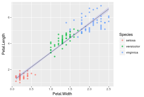
Suppose we have the famous Iris dataset, which contains measurements regarding the size of the sepal and the petal of iris flowers belonging to different types, i.e. Setosa, Versicolor, and Virginica.
Using R software, we are going to implement a linear regression to predict the length of the sepal given the petal’s width and length.
Mathematically, we are going the values a and b in the following relationship:
SepalLength = a * PetalWidth + b PetalLength +c*
The corresponding code is:
# Load required packages
library(ggplot2)
# Load iris dataset
data(iris)
# Have a look at the first 10 observations of the dataset
head(iris)
# Fit the regression line
fitted_model <- lm(Sepal.Length ~ Petal.Width + Petal.Length, data = iris)
# Get details about the parameters of the selected model
summary(fitted_model)
# Plot the data points along with the regression line
 ggplot(iris, aes(x = Petal.Width, y = Petal.Length, color = Species)) +
    geom_point(alpha = 6/10) +
    stat_smooth(method = "lm", fill="blue", colour="grey50", size=0.5, alpha = 0.1)
The results of the linear regression are shown in the following graph, where the black points represent the initial data points while the blue line the fitted regression line, which is plotted for the estimated values a = -0.31955, b = 0.54178, and c = 4.19058 that result in the best possible predictions for the target variable, i.e. the sepal length.
From now on, we will be able to make predictions regarding sepal length for new points just by applying the values of petal length and petal width into the defined linear relationship.
Logistic Regression
The main idea here is exactly the same as it was with linear regression. The difference is that the regression line is not straight anymore.
Instead, the mathematical relationship we are trying to establish is of the following form:
Y=g(a*X1+bX2)*
…where g() is the logistic function.
Due to the properties of the logistic function, Y is continuous, ranging in [0,1] and can be interpreted as the probability of an event to happen.
I know you love examples so I’ll show you one more!
This time, we will experiment with the mtcars dataset, which comprises fuel consumption and ten aspects of automobile design and performance for 32 automobiles manufactured in 1973-1974.
Using R, we are going to predict the probability of an automobile of having automatic transmission (am = 0) or manual (am = 1) based on the measurements of V/S and Miles/(US) gallon.
*am = g(a * mpg + b vs +c)**:
# Load required packages
library(ggplot2)
# Load data
data(mtcars)
# Keep a subset of the data features that includes on the measurement we are interested in
cars <- subset(mtcars, select=c(mpg, am, vs))
# Fit the logistic regression line
fitted_model <- glm(am ~ mpg+vs, data=cars, family=binomial(link="logit"))
# Plot the results
ggplot(cars, aes(x=mpg, y=vs, colour = am)) + geom_point(alpha = 6/10) +
 stat_smooth(method="glm",fill="blue", colour="grey50", size=0.5, alpha = 0.1, method.args=list(family="binomial"))
The results are shown in the following graph, where the black points represent the initial points of the dataset and the blue line the fitted logistic regression line for estimated a = 0.5359, b = -2.7957, and c = - 9.9183.

We can observe that, as mentioned before, the logistic regression output values will lie only in the range [0,1] due to the form of the regression line.
For any new automobile with given measurements for V/S and Miles/(US) gallon, we can now predict the probability that this car will have automatic transmission. Isn’t that utterly awesome?
Decision Trees
Decision trees are the second type of machine learning algorithms that we are going to investigate. They are divided in regression and classification trees, and thus can be used in supervised learning problems.
Admittedly, decision trees are one of the most intuitive algorithms, as they mimic the way people decide in many cases. What they basically do is draw a “map” of all possible paths along with the corresponding result in each case.
A graphical representation will help understand better what exactly we are talking about.
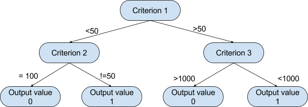
Based on a tree like this, the algorithm can decide which path to follow at each step depending on the value of the corresponding criterion. The way that the algorithm chooses the splitting criteria along with the respective thresholds at each level depends on how informative the candidate variable is for the target variable and which setup minimizes the error of the prediction produced.
Yet another example is here!
This time, the dataset under examination is readingSkills. It includes information about students who took a certain exam along with their score.
We are going to classify students into native speakers (nativeSpeaker = 1) or foreigners (nativeSpeaker= 0) based on multiple measures, including their score in the test, their shoe size, and their age.
For this implementation in R, we first need to install the party package.
# Include required packages
library(party)
library(partykit)
# Have a look at the first ten observations of the dataset
print(head(readingSkills))
input.dat <- readingSkills[c(1:105),]
# Grow the decision tree
output.tree <- ctree(
 nativeSpeaker ~ age + shoeSize + score,
 data = input.dat)
# Plot the results
plot(as.simpleparty(output.tree))
We can see that the first splitting criterion used was the score, due to its high importance in predicting the target variable, whereas shoe size wasn’t taken into consideration at all as it didn’t provide any helpful information regarding the language.

Now, if we have a new student and know their age and score on the test, we can predict whether they are a native speaker!
Clustering Algorithms
Until now, we have talked only a little bit about supervised learning problems. Now, we are moving on to the study of clustering algorithms, a subset of unsupervised learning methods.
So, just a small revision…
With clustering, if we have some initial data at our disposal, we want to form groups so that the data points belonging to some group are similar and are different from data points of the other groups.
The algorithm we are going to study is called “k-means” where k represents the number of produced clusters and is one of the most popular clustering methods.
Remember the Iris dataset we used in the example before? We are going to use it again.
For the purpose of our study, we have plotted all the data points from the dataset using their petal measures, as shown below:
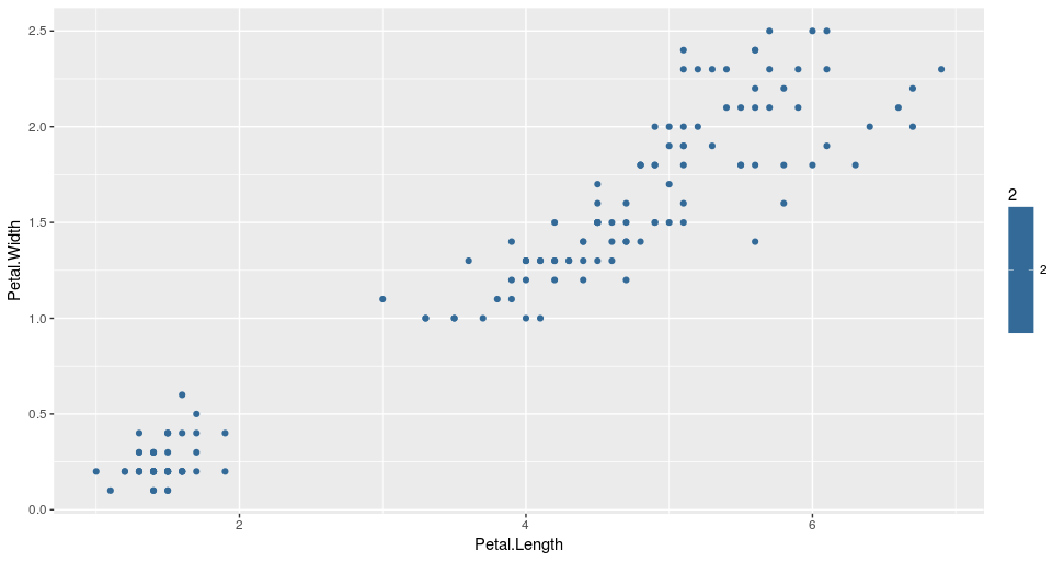
Based solely on petal measures, we are going to cluster the data points into three groups using 3-means clustering.
So how does the 3-means, or more generally, the k-means algorithm, work? The whole process can be summarized in just a few simple steps:
- Initialization step: For k=3 clusters, the algorithm randomly selects three points as centroids for each cluster.
- Cluster assignment step: The algorithm goes through the rest of the data points and assigns each one of them to the closest cluster.
- Centroid move step: After cluster assignment, the centroid of each cluster is moved to the average of all points belonging to the cluster.
Steps 2 and 3 are repeated multiple times until there is no change to be made regarding cluster assignments. The implementation of the k-means algorithm in R is easy and can be done with the following code:
# Load required packages
library(ggplot2)
library(datasets)
# Load data
data(iris)
# Set seed to make results reproducible
set.seed(20)
# Implement k-means with 3 clusters
iris_cl <- kmeans(iris[, 3:4], 3, nstart = 20)
iris_cl$cluster <- as.factor(iris_cl$cluster)
# Plot points colored by predicted cluster
ggplot(iris, aes(Petal.Length, Petal.Width, color = iris_cl$cluster)) + geom_point()
From the result, we can see that the algorithm split the data into three clusters, indicated by three different colors. We can also observe that these clusters were formed based on the size of the petals. More specifically, the red cluster includes flowers with small petals, the green cluster, iris with relatively large petals, while the blue one, iris with medium sized petals.
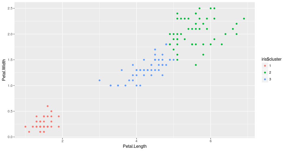
What is important to note at this point is that in any clustering, the interpretation of the formed groups requires some expert knowledge in the field. In our case, if you are not a botanist, you probably won’t realize that what the k-means managed to do is cluster the iris into their different types, i.e. Setosa, Versicolor, and Virginica without having any knowledge about them!
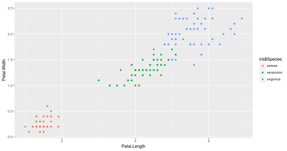
So if we plot the data again, this time colored by their species, we will see the similarity in the clusters.
Summary
We have come a long way from where we began. We’ve talked about regression (both linear and logistic), decision trees, and finally, k-means clustering. We also set up some simple, yet powerful, implementations of each one of these methods in R.
So, what are the advantages of each algorithm over the others? Which one should you choose for a real-life problem?
Firstly, the presented methods are not some toy algorithms — they are widely used in production systems around the world, and so depending on the task, they can be pretty powerful.
Secondly, in order to answer the above question, you have to be clear what exactly you mean by advantages, as the relative benefits of each method can be expressed in many contexts, i.e. interpretability, robustness, computational time, etc.
Assuming that for the time being, we care only about the method’s appropriateness and predictive performance, a short summary of each method’s pros and cons follows:

Now, we are finally ready to confidently implement this knowledge to some real-world problems!
#machine-learning #python #data-science