Overview

One of the most popular ways of representing and forecasting time series data is through Autoregressive Integrated Moving Average (ARIMA) models. These models are defined by three parameters:

• p: the lag order (number of lag observations included)
• d: the degree of differencing needed for stationarity (number of times the data is differenced)
• q: the order of the moving average

If you’re new to ARIMA modeling, there are lots of great instructional webpages and step-by-step guides such as this one from otexts.com and this one on oracle.com which give more thorough overviews.

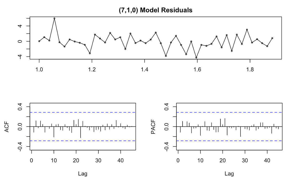
However, the vast majority of these guides suggest setting the p, d, and q parameters by using the auto.arima() function or by hand using ACF and PACF plots. As someone who frequently uses ARIMA models, I felt like I still needed a better option. The models suggested to me by auto.arima() frequently had high AIC values (a measure for comparing models — the best model is typically that with the lowest AIC) and significant lags which indicate poor model fit. While I could achieve lower AIC values and eliminate significant lags by changing parameters by hand, this process felt somewhat arbitrary and I was never confident that I was truly selecting the best possible model for my data.

I eventually began using grid searches to aid my selection of parameters. While it’s always important to conduct exploratory analyses with your data, test assumptions, and think critically about the ACF and PACF plots, I have found it very useful to have a data-driven place to start with my parameter selection. I will walk through example code and output comparing the auto.arima() and grid search approaches below.

#arima #data-science #time-series-analysis #grid-search #r