Before Starting the blog lets us refresh some of the basic definitions
What is machine Learning?
“Machine learning (ML) is the study of computer algorithms that improve automatically through experience.It is seen as a subset of artificial intelligence. Machine learning algorithms build a mathematical model based on sample data, known as “training data”, in order to make predictions or decisions without being explicitly programmed to do so .Machine learning algorithms are used in a wide variety of applications, such as email filtering and computer vision.”
source: Wikipedia
As, per the above definition the models require training data to compute predictions. Depending upon the data provided the machine learning algorithm can be broadly classified into 3 categories namely supervised, unsupervised and semi supervised learning.
In this blog, we are going to learn about one such supervised learning algorithm.
Supervised Algorithms basically can be divided into two categories:
Classification:
In this type of problem the machine learning algorithm will specify the data belongs to which set of class. The classes can be binary as well as multiple class.
E.g. Logistic Regression, Decision Tree, Random Forest, Naïve Bayes.
Regression:
In this type of problems the machine learning algorithm will try to find the relationship between continuous of variables. The modelling approach used here is between a dependent variable (response variable) with a given set of independent (feature) variables. Just fyi I will be using Response and target variable’s interchangeably along with LR for Linear Regression.
E.g. Linear Regression, Ridge Regression, Elastic Net Regression.
Today we are going to learn Simple Linear Regression.
Linear Regression:
I personally believe to learn any machine learning model or any concept related to it if we understand the geometric intuition behind it then it will stay longer with us as visuals helps sustain memory as compared to a mathematical representation.
So, to proceed with the blog we will be categorizing into below aspects for LR:
1. What is Linear Regression?
2. Geometric Intuition
3. Optimization Problem
4. Implementation with sklearn Library.
What is Linear Regression?
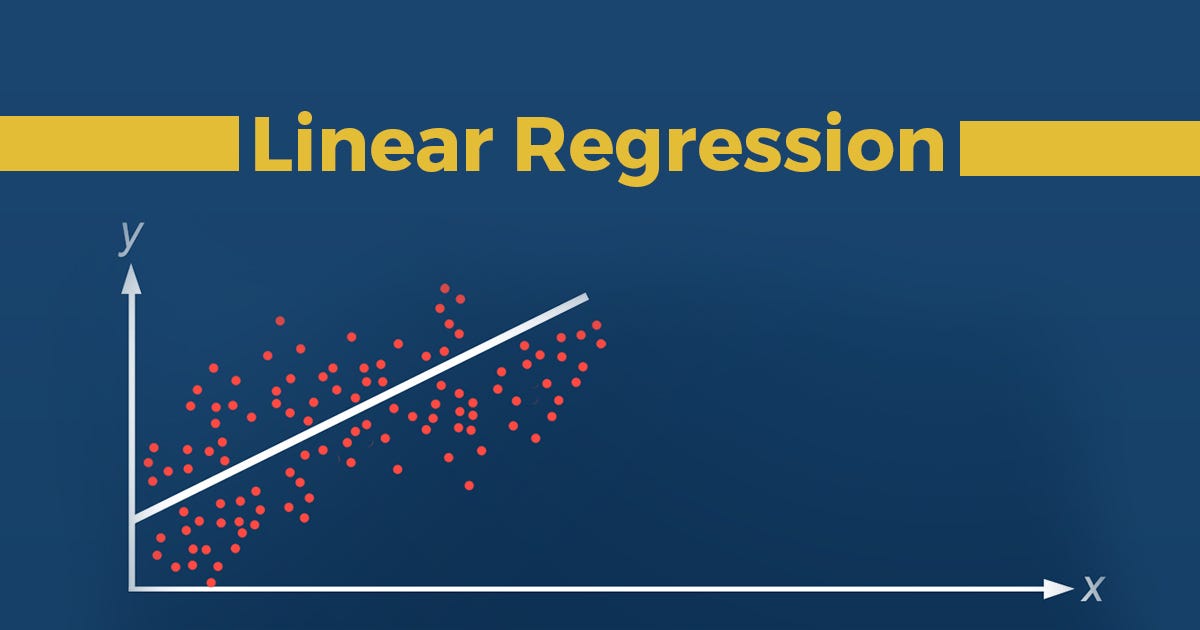
As stated, above LR is a type of Regression Technique which tries to find relation between continuous set of variables from any given dataset.
So, the problem statement that algorithm tries to solve linearly is to best fit a line/plane/hyperplane (as the dimension goes on increasing) for any given set of data. Yes, It’s that simple
We understand this with the help of below scatter Plot.
Geometric Intuition:
To represent visually let’s take a look at below scatter plot which is derived from Boston Housing Data set which I have used as an example in the latter part of the blog.
The co-ordinates are denoted as below,
X-Axis -> Actual House Prices
Y-Axis -> Predicted house Prices

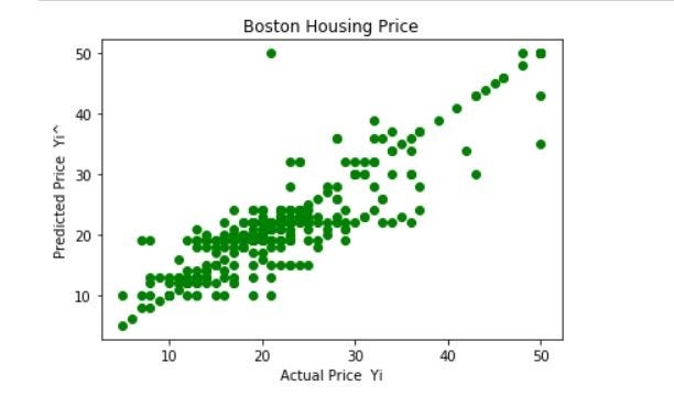
Figure -1
People I want you to stay with me on this as we need to try to understand what LR is doing visually So, having a look at the scatter plot if we visualize and try to pass an imaginary line from the origin then the line will be passing from most the predicted points which shows that model has correctly plotted most of the response variables.
Optimization Problem:
Now, as we are getting hold of what LR does visually let’s have a look at the optimization problem that we are going to solve because every machine learning algorithm boil’s down to an optimization problem where we can understand the crux of it through a mathematical equation.
For any Machine learning algo the ultimate goal is to reduce the error’s in the dataset so that it can predict the target variable’s more accurately.
With that said what is the optimization problem for Linear Regression? Which is used to minimize sum of errors across the Training data. The next question which will pop up in your mind is why sum of errors?

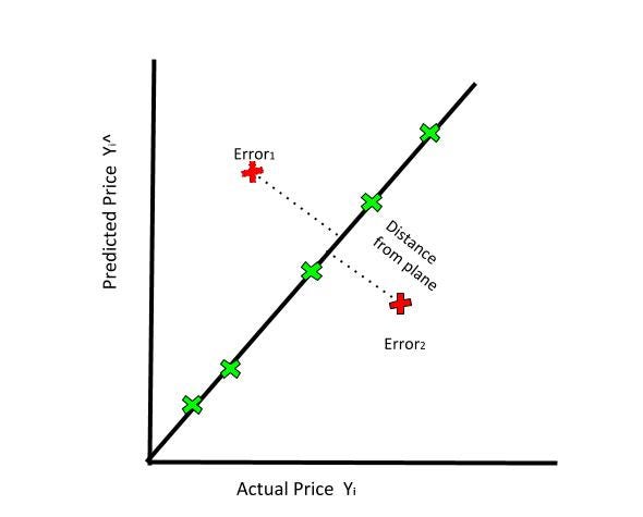
The above image which is a lighter version of the scatter plot answers that question perfectly, so as you can see we have drawn a line passing through the origin which will have the points which are correctly classified denoted by green cross. But also, if we look closely there are few of the points which are not present on that line denoted by red cross. These points can be differentiated as points above and below that line. These points can be defined as data point which the model was not able to predict it correctly. And the optimization problem is used to reduce the distance of these error points.
#linear-regression #beginners-guide #machine-learning #deep learning