Analyzing time series is such a useful resource for essentially any business, data scientists entering the field should bring with them a solid foundation in the technique. Here, we decompose the logical components of a time series using R to better understand how each plays a role in this type of analysis.
By Omar Martinez, Arcalea.
Analyzing time series can be an extremely useful resource for virtually any business, therefore, it is extremely important for data scientists entering the field to have a solid foundation on the main concepts. Luckily, a time series can be decomposed into its different elements and the decomposition of the process allows us to understand each of the parts that play a role in the analysis as a logical component of the whole system.
While it is true that R has already many powerful packages to analyze time series, in this article the goal is to perform a time series analysis --specifically for forecasting-- by building a function from scratch to analyze each of the different elements in the process.
What are the elements of a time series?
There are several methods to do forecasting, but in this article, we’ll focus on the multiplicative time series approach, in which we have the following elements:
**Seasonality: **It consists of variations that occur at regular intervals, for example, every quarter, on summer vacation, at the end of the year, etc. A clear example would be higher conversion rates on gym memberships in January or a spike in video game sales around the holidays.
**Trend: **It can be categorized as a general tendency of the data to either decrease or increase during a longer period, for example, in the stock market, generally a “bear market” on average could be marked by a general decrease in stock values for a period of around two years. Of course, this is an oversimplification, but we get the idea.
**Irregular Component: **You can think of the irregular component as the residual time series after the previous two components have been removed. The irregular component corresponds to the frequency fluctuations of the series.
With these components, we can create a model in the following way:
_Y i _= _Si _* _T i _* Ii
Implementing this in R is relatively straight forward, so let’s open a new notebook, and let us write some code.
Time series forecasting in R
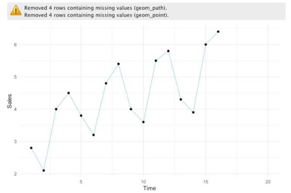
To start, let’s create a data frame with the data we’ll be analyzing. Suppose that you are looking at data on sales over time and that you have total sales vales by quarter.
x<-seq(1, 20)
y<-c(2.8, 2.1, 4, 4.5, 3.8, 3.2, 4.8, 5.4, 4, 3.6, 5.5, 5.8, 4.3, 3.9, 6, 6.4, NA, NA, NA, NA)
data <- data.frame(t=x, sales=y)
data
To provide more context, in the snippet above, we are creating an array of sales by quarter for five years. Notice that we have included four “NA”s, these are the values we are going to forecast. Because we are looking at quarterly data, this means that we’ll be forecasting year five.
#2020 jul tutorials #overviews #beginners #r #time series #data analysis