Learn the basics of classification with guided code from the iris data set

When I was first learning how to code, I would practice my data skills on different data sets to create mini Jupyter Notebook reference guides. Since I have found this to be an incredibly useful tool, I thought I’d start sharing code walk-throughs. Hopefully this is a positive resource for those learning to use Python for data science, and something that can be referenced in future projects. Full code is available on Github.

Getting Set Up

The first step is to import the preloaded data sets from the scikit-learn python library. More info on the “toy” data sets included in the package can be found here. The data description will also give more information on the features, statistics, and sources.

from sklearn.datasets import load_iris

#save data information as variable
iris = load_iris()
#view data description and information
print(iris.DESCR)

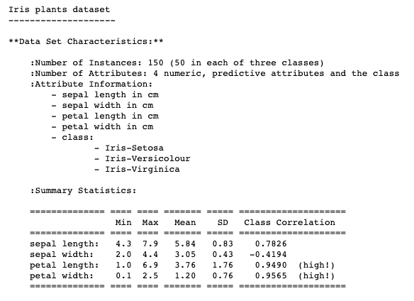
The data will be pre-saved as a dictionary with the keys “data” and “target”, each paired with an array of lists as the values. Initially the information will be output like this:

{'data': array([[5.1, 3.5, 1.4, 0.2],
        [4.9, 3\. , 1.4, 0.2],
        [4.7, 3.2, 1.3, 0.2],
        [4.6, 3.1, 1.5, 0.2],
        [5\. , 3.6, 1.4, 0.2],
        [5.4, 3.9, 1.7, 0.4],
        [4.6, 3.4, 1.4, 0.3] ...
'target': array([0, 0, 0, 0, 0, 0, 0, 0, 0, 0, 0, 0 ...}

Putting Data into a Data Frame

Feature Data

To view the data more easily we can put this information into a data frame by using the Pandas library. Let’s create a data frame to store the data information about the flowers’ features first.

import pandas as pd

#make sure to save the data frame to a variable
data = pd.DataFrame(iris.data)
data.head()

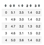
Using data.head() will automatically output the first 5 rows of data, but if we can also specify how many rows we want in the brackets, data.head(10).

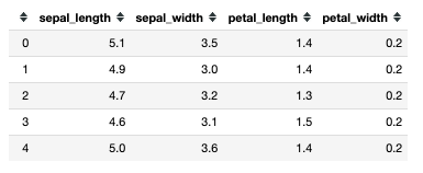
Now, we have a data frame with the iris data, but the columns are not clearly labeled. Looking at the data description we printed above, or referencing the source code tells us more about the features. In the documentation the data features are listed as:

• sepal length in cm
• sepal width in cm
• petal length in cm
• petal width in cm

Let’s rename the columns so the features are clear.

data.columns = ['sepal_length', 'sepal_width', 'petal_length', 'petal_width']

#note: it is common practice to use underscores between words, and avoid spaces
data.head()

Target Data

Now that the data related to the features is neatly in a data frame, we can do the same with the target data.

#put target data into data frame
target = pd.DataFrame(iris.target)

#Lets rename the column so that we know that these values refer to the target values
target = target.rename(columns = {0: 'target'})
target.head()

The target data frame is only one column, and it gives a list of the values 0, 1, and 2. We will use the information from the feature data to predict if a flower belongs in group 0, 1, or 2. But what do these numbers refer to?

• 0 is Iris Setosa
• 1 is Iris Versicolour
• 2 is Iris Virginica

Exploratory Data Analysis (EDA)

To help us understand our data better, let’s first combine the two data frames we just created. By doing this we can see the features and class determination of the flowers together.

df = pd.concat([data, target], axis = 1)

#note: it is common practice to name your data frame as "df", but you can name it anything as long as you are clear and consistent
#in the code above, axis = 1 tells the data frame to add the target data frame as another column of the data data frame, axis = 0 would add the values as another row on the bottom
df.head()

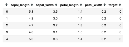
Now we can clearly see the relationship between an individual flower’s features and its class.

Data Cleaning

It’s super important to look through your data, make sure it is clean, and begin to explore relationships between features and target variables. Since this is a relatively simple data set there is not much cleaning that needs to be done, but let’s walk through the steps.

1. Look at Data Types

df.dtypes

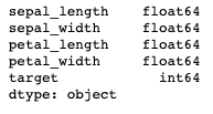
float = numbers with decimals (1.678)

int = integer or whole number without decimals (1, 2, 3)

obj = object, string, or words (‘hello’)

The 64 after these data types refers to how many bits of storage the value occupies. You will often seen 32 or 64.

In this data set, the data types are all ready for modeling. In some instances the number values will be coded as objects, so we would have to change the data types before performing statistic modeling.

2. Check for Missing Values

df.isnull().sum()

This data set is not missing any values. While this makes modeling much easier, this is not usually the case — data is always messy in real life. If there were missing values you could delete rows of data that had missing values, or there are several options of how you could fill that missing number (with the column’s mean, previous value…).

#exploratory-data-analysis #logistic-regression #data-science #basics #classification #data analysis