Top 10 Machine Learning Algorithms You Need to Know
The use of Machine Learning and its prowess had grown exponentially over the last few years. The things our grandparents thought could only be done by an intellectual human are now being done by machines without human interference. Such is the power of Machine Learning.
Arthur Samuel of IBM when first came up with the phrase “Machine Learning” in 1952 for his game of checkers, he would have never thought that Machine Learning would open up a whole new spectrum from helping people with disabilities to felicitating businesses with decision-making and dynamic pricing.
Machine learning is a method of data analysis that automates analytical model building. It is a branch of technology that allows systems to learn from data, identify patterns and make decisions with minimal human intervention.
Machine Learning made it possible to build software that can understand images, sounds, and language and for us to learn more about technology each day.
When I first came to know about Machine Learning from an article in Verge in 2013, I could never understand how can machines be trained!?? It was not until I began my undergrad in 2015 and I began to learn Machine Learning. Training data, test data, supervised-unsupervised data, decision trees, random forests to deep learning and neural networks, it was a heavy cloud of knowledge.
One after the other, I learned the different Machine Learning algorithms and did projects about it. The more I read and worked with them, I understand that there are some algorithms you start off with and that makes you more familiar with the whole ML and AI ecosystem.
Before we get into the story, it is extremely important to set the base correct on supervised, unsupervised learning and Reinforcement learning.
Types of Machine Learning Algorithms
There are 3 types of machine learning (ML) algorithms:
Supervised Learning Algorithms:
Supervised learning uses labeled training data to learn the mapping function that turns input variables (X) into the output variable (Y). In other words, it solves for f in the following equation:
This allows us to accurately generate outputs when given new inputs.
We’ll talk about two types of supervised learning: classification and regression.
Classification is used to predict the outcome of a given sample when the output variable is in the form of categories. A classification model might look at the input data and try to predict labels like “sick” or “healthy.”
Regression is used to predict the outcome of a given sample when the output variable is in the form of real values. For example, a regression model might process input data to predict the amount of rainfall, the height of a person, etc.
The first 5 algorithms that we cover in this blog – Linear Regression, Logistic Regression, CART, Naïve-Bayes, and K-Nearest Neighbors (KNN) — are examples of supervised learning.
Ensembling is another type of supervised learning. It means combining the predictions of multiple machine learning models that are individually weak to produce a more accurate prediction on a new sample. Algorithms 9 and 10 of this article — Bagging with Random Forests, Boosting with XGBoost — are examples of ensemble techniques.
Unsupervised Learning Algorithms:
Unsupervised learning models are used when we only have the input variables (X) and no corresponding output variables. They use unlabeled training data to model the underlying structure of the data.
We’ll talk about three types of unsupervised learning:
Association is used to discover the probability of the co-occurrence of items in a collection. It is extensively used in market-basket analysis. For example, an association model might be used to discover that if a customer purchases bread, s/he is 80% likely to also purchase eggs.
Clustering is used to group samples such that objects within the same cluster are more similar to each other than to the objects from another cluster.
Dimensionality Reduction is used to reduce the number of variables of a data set while ensuring that important information is still conveyed. Dimensionality Reduction can be done using Feature Extraction methods and Feature Selection methods. Feature Selection selects a subset of the original variables. Feature Extraction performs data transformation from a high-dimensional space to a low-dimensional space. Example: PCA algorithm is a Feature Extraction approach.
Algorithms 6-8 that we cover here — Apriori, K-means, PCA — are examples of unsupervised learning.
Reinforcement learning:
Reinforcement learning is a type of machine learning algorithm that allows an agent to decide the best next action based on its current state by learning behaviors that will maximize a reward.
Reinforcement algorithms usually learn optimal actions through trial and error. Imagine, for example, a video game in which the player needs to move to certain places at certain times to earn points. A reinforcement algorithm playing that game would start by moving randomly but, over time through trial and error, it would learn where and when it needed to move the in-game character to maximize its point total.
So, with this story from me, let’s get into the Top 10 Machine Learning Algorithms that we have heard about a hundred times, but read with clarity this time about its applications and powers, in no particular order of importance.
1. Linear Regression
In machine learning, we have a set of input variables (x) that are used to determine an output variable (y). A relationship exists between the input variables and the output variable. The goal of ML is to quantify this relationship.
Figure 1: Linear Regression is represented as a line in the form of y = a + bx. Source
In Linear Regression, the relationship between the input variables (x) and output variable (y) is expressed as an equation of the form y = a + bx. Thus, the goal of linear regression is to find out the values of coefficients a and b. Here, a is the intercept and b is the slope of the line.
Figure 1 shows the plotted x and y values for a data set. The goal is to fit a line that is nearest to most of the points. This would reduce the distance (‘error’) between the y value of a data point and the line.
2. Logistic Regression
Linear regression predictions are continuous values (i.e., rainfall in cm), logistic regression predictions are discrete values (i.e., whether a student passed/failed) after applying a transformation function.
Logistic regression is best suited for binary classification: data sets where y = 0 or 1, where 1 denotes the default class. For example, in predicting whether an event will occur or not, there are only two possibilities: that it occurs (which we denote as 1) or that it does not (0). So if we were predicting whether a patient was sick, we would label sick patients using the value of 1 in our data set.
Logistic regression is named after the transformation function it uses, which is called the logistic function h(x)= 1/ (1 + ex). This forms an S-shaped curve.
In logistic regression, the output takes the form of probabilities of the default class (unlike linear regression, where the output is directly produced). As it is a probability, the output lies in the range of 0-1. So, for example, if we’re trying to predict whether patients are sick, we already know that sick patients are denoted as 1, so if our algorithm assigns the score of 0.98 to a patient, it thinks that patient is quite likely to be sick.
This output (y-value) is generated by log transforming the x-value, using the logistic function h(x)= 1/ (1 + e^ -x) . A threshold is then applied to force this probability into a binary classification.
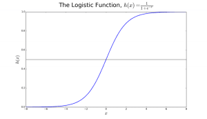
Figure 2: Logistic Regression to determine if a tumor is malignant or benign. Classified as malignant if the probability h(x)>= 0.5. Source
In Figure 2, to determine whether a tumor is malignant or not, the default variable is y = 1 (tumor = malignant). The x variable could be a measurement of the tumor, such as the size of the tumor. As shown in the figure, the logistic function transforms the x-value of the various instances of the data set, into the range of 0 to 1. If the probability crosses the threshold of 0.5 (shown by the horizontal line), the tumor is classified as malignant.
The logistic regression equation P(x) = e ^ (b0 +b1x) / (1 + e(b0 + b1x)) can be transformed into ln(p(x) / 1-p(x)) = b0 + b1x.
The goal of logistic regression is to use the training data to find the values of coefficients b0 and b1 such that it will minimize the error between the predicted outcome and the actual outcome. These coefficients are estimated using the technique of Maximum Likelihood Estimation.
3. CART
Classification and Regression Trees (CART) are one implementation of Decision Trees.
The non-terminal nodes of Classification and Regression Trees are the root node and the internal node. The terminal nodes are the leaf nodes. Each non-terminal node represents a single input variable (x) and a splitting point on that variable; the leaf nodes represent the output variable (y). The model is used as follows to make predictions: walk the splits of the tree to arrive at a leaf node and output the value present at the leaf node.
The decision tree in Figure 3 below classifies whether a person will buy a sports car or a minivan depending on their age and marital status. If the person is over 30 years and is not married, we walk the tree as follows : ‘over 30 years?’ -> yes -> ’married?’ -> no. Hence, the model outputs a sports car.
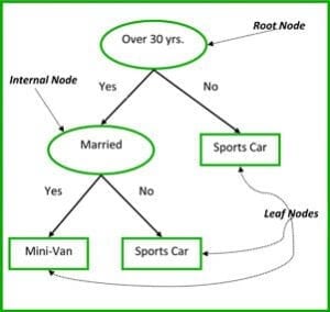
Figure 3: Parts of a decision tree. Source
4. Naïve Bayes
To calculate the probability that an event will occur, given that another event has already occurred, we use Bayes’s Theorem. To calculate the probability of hypothesis(h) being true, given our prior knowledge(d), we use Bayes’s Theorem as follows:
where:
- P(h|d) = Posterior probability. The probability of hypothesis h being true, given the data d, where P(h|d)= P(d1| h) P(d2| h)….P(dn| h) P(d)
- P(d|h) = Likelihood. The probability of data d given that the hypothesis h was true.
- P(h) = Class prior probability. The probability of hypothesis h being true (irrespective of the data)
- P(d) = Predictor prior probability. Probability of the data (irrespective of the hypothesis)
This algorithm is called ‘naive’ because it assumes that all the variables are independent of each other, which is a naive assumption to make in real-world examples.
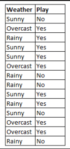
Figure 4: Using Naive Bayes to predict the status of ‘play’ using the variable ‘weather’.
Using Figure 4 as an example, what is the outcome if weather = ‘sunny’?
To determine the outcome play = ‘yes’ or ‘no’ given the value of variable weather = ‘sunny’, calculate P(yes|sunny) and P(no|sunny) and choose the outcome with higher probability.
->P(yes|sunny)= (P(sunny|yes) * P(yes)) / P(sunny) = (3/9 * 9/14 ) / (5/14) = 0.60
-> P(no|sunny)= (P(sunny|no) * P(no)) / P(sunny) = (2/5 * 5/14 ) / (5/14) = 0.40
Thus, if the weather = ‘sunny’, the outcome is play = ‘yes’.
5. KNN
The K-Nearest Neighbors algorithm uses the entire data set as the training set, rather than splitting the data set into a training set and test set.
When an outcome is required for a new data instance, the KNN algorithm goes through the entire data set to find the k-nearest instances to the new instance, or the k number of instances most similar to the new record, and then outputs the mean of the outcomes (for a regression problem) or the mode (most frequent class) for a classification problem. The value of k is user-specified.
The similarity between instances is calculated using measures such as Euclidean distance and Hamming distance.
Unsupervised learning algorithms
6. Apriori
The Apriori algorithm is used in a transactional database to mine frequent item sets and then generate association rules. It is popularly used in market basket analysis, where one checks for combinations of products that frequently co-occur in the database. In general, we write the association rule for ‘if a person purchases item X, then he purchases item Y’ as : X -> Y.
Example: if a person purchases milk and sugar, then she is likely to purchase coffee powder. This could be written in the form of an association rule as: {milk,sugar} -> coffee powder. Association rules are generated after crossing the threshold for support and confidence.
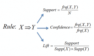
Figure 5: Formulae for support, confidence and lift for the association rule X->Y.
The Support measure helps prune the number of candidate item sets to be considered during frequent item set generation. This support measure is guided by the Apriori principle. The Apriori principle states that if an itemset is frequent, then all of its subsets must also be frequent.
7. K-means
K-means is an iterative algorithm that groups similar data into clusters.It calculates the centroids of k clusters and assigns a data point to that cluster having least distance between its centroid and the data point.
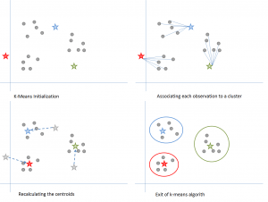
Figure 6: Steps of the K-means algorithm. Source
Here’s how it works:
We start by choosing a value of k. Here, let us say k = 3. Then, we randomly assign each data point to any of the 3 clusters. Compute cluster centroid for each of the clusters. The red, blue and green stars denote the centroids for each of the 3 clusters.
Next, reassign each point to the closest cluster centroid. In the figure above, the upper 5 points got assigned to the cluster with the blue centroid. Follow the same procedure to assign points to the clusters containing the red and green centroids.
Then, calculate centroids for the new clusters. The old centroids are gray stars; the new centroids are the red, green, and blue stars.
Finally, repeat steps 2-3 until there is no switching of points from one cluster to another. Once there is no switching for 2 consecutive steps, exit the K-means algorithm.
8. PCA
Principal Component Analysis (PCA) is used to make data easy to explore and visualize by reducing the number of variables. This is done by capturing the maximum variance in the data into a new coordinate system with axes called ‘principal components’.
Each component is a linear combination of the original variables and is orthogonal to one another. Orthogonality between components indicates that the correlation between these components is zero.
The first principal component captures the direction of the maximum variability in the data. The second principal component captures the remaining variance in the data but has variables uncorrelated with the first component. Similarly, all successive principal components (PC3, PC4 and so on) capture the remaining variance while being uncorrelated with the previous component.
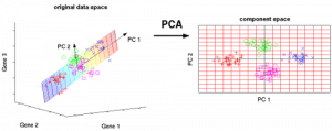
Figure 7: The 3 original variables (genes) are reduced to 2 new variables termed principal components (PC’s). Source
Ensemble learning techniques:
Ensembling means combining the results of multiple learners (classifiers) for improved results, by voting or averaging. Voting is used during classification and averaging is used during regression. The idea is that ensembles of learners perform better than single learners.
9. Bagging with Random Forests
The first step in bagging is to create multiple models with data sets created using the Bootstrap Sampling method. In Bootstrap Sampling, each generated training set is composed of random subsamples from the original data set.
Each of these training sets is of the same size as the original data set, but some records repeat multiple times and some records do not appear at all. Then, the entire original data set is used as the test set. Thus, if the size of the original data set is N, then the size of each generated training set is also N, with the number of unique records being about (2N/3); the size of the test set is also N.
The second step in bagging is to create multiple models by using the same algorithm on the different generated training sets.
This is where Random Forests enter into it. Unlike a decision tree, where each node is split on the best feature that minimizes error, in Random Forests, we choose a random selection of features for constructing the best split. The reason for randomness is: even with bagging, when decision trees choose the best feature to split on, they end up with similar structure and correlated predictions. But bagging after splitting on a random subset of features means less correlation among predictions from subtrees.
The number of features to be searched at each split point is specified as a parameter to the Random Forest algorithm.
Thus, in bagging with Random Forest, each tree is constructed using a random sample of records and each split is constructed using a random sample of predictors.
10. Boosting with AdaBoost
Adaboost stands for Adaptive Boosting. Bagging is a parallel ensemble because each model is built independently. On the other hand, boosting is a sequential ensemble where each model is built based on correcting the misclassifications of the previous model.
Bagging mostly involves ‘simple voting’, where each classifier votes to obtain a final outcome– one that is determined by the majority of the parallel models; boosting involves ‘weighted voting’, where each classifier votes to obtain a final outcome which is determined by the majority– but the sequential models were built by assigning greater weights to misclassified instances of the previous models.
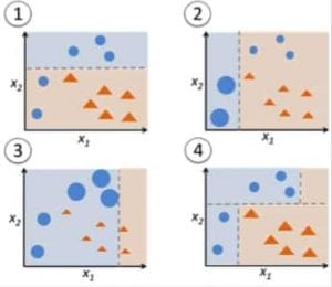
Figure 9: Adaboost for a decision tree. Source
In Figure 9, steps 1, 2, 3 involve a weak learner called a decision stump (a 1-level decision tree making a prediction based on the value of only 1 input feature; a decision tree with its root immediately connected to its leaves).
The process of constructing weak learners continues until a user-defined number of weak learners has been constructed or until there is no further improvement while training. Step 4 combines the 3 decision stumps of the previous models (and thus has 3 splitting rules in the decision tree).
First, start with one decision tree stump to make a decision on one input variable.
The size of the data points show that we have applied equal weights to classify them as a circle or triangle. The decision stump has generated a horizontal line in the top half to classify these points. We can see that there are two circles incorrectly predicted as triangles. Hence, we will assign higher weights to these two circles and apply another decision stump.
Second, move to another decision tree stump to make a decision on another input variable.
We observe that the size of the two misclassified circles from the previous step is larger than the remaining points. Now, the second decision stump will try to predict these two circles correctly.
As a result of assigning higher weights, these two circles have been correctly classified by the vertical line on the left. But this has now resulted in misclassifying the three circles at the top. Hence, we will assign higher weights to these three circles at the top and apply another decision stump.
Third, train another decision tree stump to make a decision on another input variable.
The three misclassified circles from the previous step are larger than the rest of the data points. Now, a vertical line to the right has been generated to classify the circles and triangles.
Fourth, Combine the decision stumps.
We have combined the separators from the 3 previous models and observe that the complex rule from this model classifies data points correctly as compared to any of the individual weak learners.
Conclusion:
To recap, we have covered some of the the most important machine learning algorithms for data science:
- 5 supervised learning techniques- Linear Regression, Logistic Regression, CART, Naïve Bayes, KNN.
- 3 unsupervised learning techniques- Apriori, K-means, PCA.
- 2 ensembling techniques- Bagging with Random Forests, Boosting with XGBoost.
#machinelearning #datascience #python #tensorflow