Originally I wanted to write a single article for a fair comparison of Pandas and Spark, but it continued to grow until I decided to split this up. This is the second part of the small series.

• Spark vs Pandas, part 1 — Pandas
• Spark vs Pandas, part 2 — Spark
• Spark vs Pandas, part 3 — Programming Languages
• Spark vs Pandas, part 4 — Shootout and Recommendation

What to Expect

This second part portrays Apache Spark. I already wrote a different article about Spark as part of a series about Big Data Engineering, but this time I will focus more on the differences to Pandas.

What is Apache Spark?

Apache Spark is a Big Data processing framework written in Scala targeting the Java Virtual Machine, but which also provides language bindings for Java, Python and R. The inception of Spark is probably very different from Pandas, since Spark initially mainly addressed the challenge of efficiently working with huge amounts of data, which do not fit into the memory of a single computer (or even into the total amount of memory of a whole computing cluster) any more.

One can say that Spark was created to replace Hadoop MapReduce by providing both a simpler and at the same time more powerful programming model. And Spark was very successful with that mission, since I assume that no project would start writing new Hadoop MapReduce jobs by today and clearly go with Spark instead.

Spark Data Model

Initially Spark only provided a (nowadays called low level) API called RDDs, which required developers to model their data as classes. After a couple of years, Spark was extended by the DataFrame API which picked up many of the good ideas of Pandas and R and which is now the preferred API to use (together with DataSets, but I’ll omit them in this discussion).

Similar to Pandas, Spark DataFrames are built on the concepts of columns and rows, with the set of columns implicitly defining a schema which is shared among all rows.

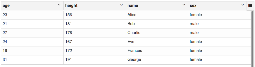
A Spark DataFrame with multiple columns

In contrast to Pandas, the schema definition of a Spark DataFrame also dictates the data type for each column that can be stored in each row. This aspect strongly resembles classical databases, where each column also has a fixed data type which is enforced on all records (newer NoSQL databases might be more flexible, but that doesn’t mean that type enforcement is bad or old-school). You can easily display the schema of a given DataFrame, in order to inspect the columns and their data types:

Schema of the DataFrame above

As opposed to Pandas, Spark doesn’t support any indexing for efficient access to individual rows in a DataFrame. Spark solves all tasks which could benefit from an index more or less by brute-force —since all transformations are always performed on all records, Spark will reorganize the data as needed on the fly.

Generally speaking, columns and rows in Spark are not interchangeable like they are in Pandas. The reason for this lack of orthogonality is that Spark is designed to scale with data in terms of number of rows, but not in terms of number of columns. Spark can easily work with billions of rows, but the number of columns should always be limited (hundreds or maybe a couple of thousands).

When we try to model stock prices with open, close, low, high and volume attributes, we therefore need to take a different approach in Spark than in Pandas. Instead of using wide DataFrames with different columns for different stocks, we use a more normalized (in the sense database normalization) approach where each row is uniquely identified by its dimensions date and asset and contains the metrics close, high, low and open.

DataFrame containing stock numbers

Although the data model of Apache Spark is less flexible than the one of Pandas, that doesn’t need to be a bad thing. These restrictions naturally arise with Sparks focus on implementing a relational algebra (more on that below) and the enforcement of strict data types help you to find bugs on your side earlier.

Since Spark doesn’t support indices, it also doesn’t support nested indices like Pandas. Instead Spark offers very good support for deeply nested data structures, like they are found in JSON documents or Avro messages. These kinds of data are often used in internal communication protocols between applications and Sparks exhaustive support of them underlines its focus as a data processing tool. Nested structures are implemented as complex data types like structs, arrays and maps, which in turn can again contain these complex data types.

As an example, I show you some Twitter data, which is publicly available on the Internet Archive.

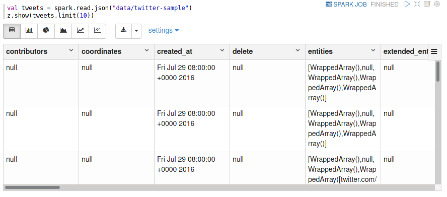
Nested data shown in tabular form

This tabular representation doesn’t really show the complex nature of the tweets. A look at the schema reveals all details (although only a subsection is shown below):

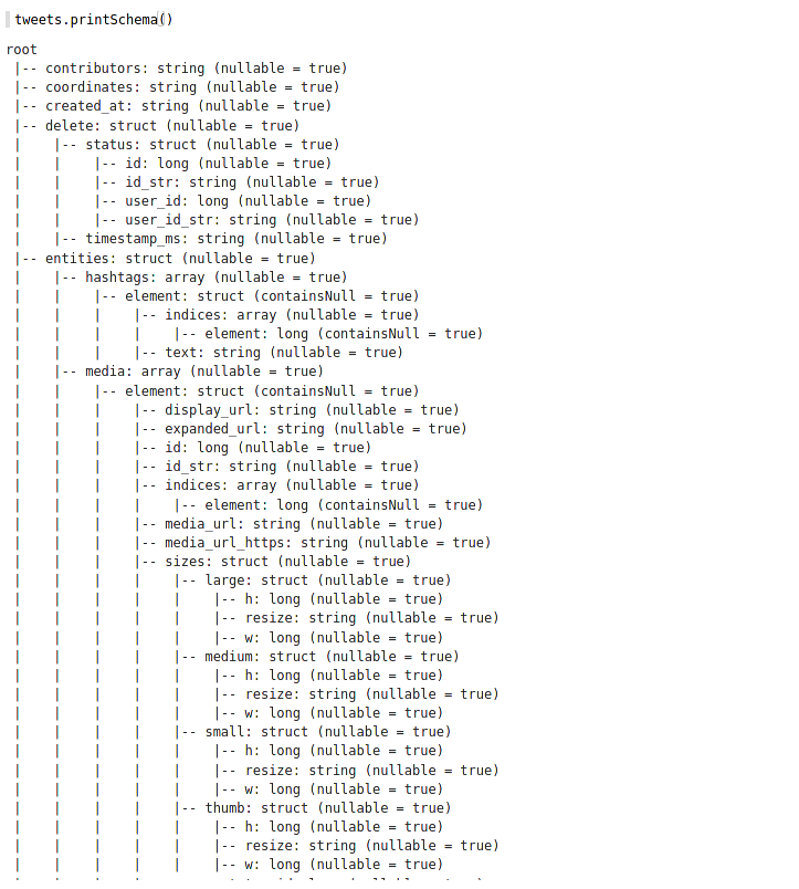
Part of the full schema of the twitter data set

This sort of support for complex and deeply nested schemas is something which sets Spark apart from Pandas, which can only work with purely tabular data. And since this type of data naturally arises in many domains, it is good to know that Spark could be a tool for working with that data. Suggestions for working with this kind of data might be an interesting topic for a separate article.

Flexibility of Spark

Apache Spark also provides a broad set of transformations, which implement a full relational algebra as you find in traditional databases (MySQL, Oracle, DB2, MS SQL, …). This means that you can perform just any transformation like you could do within a SELECT statement in SQL.

The Spark/Scala examples below follow along the lines of the Pandas examples in the first article. Note how Spark uses the wording (but not the syntax) of SQL in all its methods.

Projections

One of the possibly simplest transformations is a projection, which simply creates a new DataFrame with a subset of the existing columns. This operation is called projection, because it is similar to a mathematical projection of a higher-dimensional space into a lower dimensional space (for example 3d to 2d). Specifically a projection reduces the number of dimensions and it is idempotent, i.e. performing the same projection a second time on the result will not change the data any more.

A projection in SQL would be a very simple SELECT statement with a subset of all available columns. Note how the name of the Spark method select reflects this equivalence.

Filtering

The next simple transformation in filtering, which only selects a subset of the available rows.

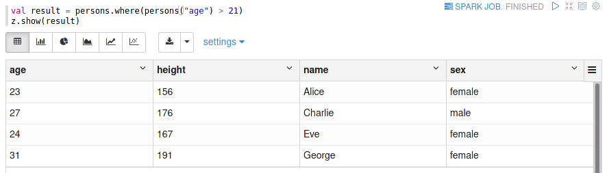
Selecting people, which are older than 21 years.

Filtering in SQL is typically performed within the WHERE clause. Again note that Spark chose to use the SQL term where although Scala users would prefer filter — actually you can also use the equivalent method filter instead.

Joins

Joins are an elementary operation in a relation database — without them, the term relational wouldn’t be very meaningful.

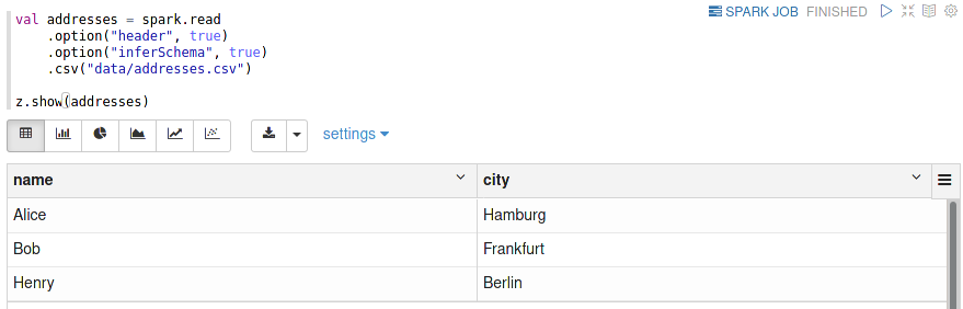
For a small demonstration, I first load a second DataFrame containing the name of the city some persons live in:

Now we can now perform the join operation:

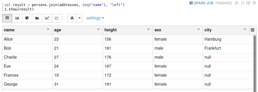
In SQL a join operation is performed via the JOIN clause as part of a SELECT statement.

Note that as opposed to Pandas, Spark does not require special indexing of either DataFrames (if you remember, Spark doesn’t support the concept of indices).

Instead of relying on usable indices, Spark will reorganize the data under the hood as part of implementing an efficient parallel and distributed join operation. This reorganization will shuffle the data among all machines of a cluster, which means that all records of both DataFrames will be redistributed such that records with matching join keys are sent to the same machine. Once this shuffle phase is done, the join can be executed independently in parallel using a sort-merge join on all machines.

#spark #pandas #python #data-science #developer