Statistics play an important role in our lives. It eventually becomes an imperative fundamental of any data scientist. Today we are about to review some basic concepts in hypothesis tests with a scenario as below.
Scenario
Imagine on a hot day, you’re going down the street and then stop at a watermelon store. The fruits there look so good that you immediately decide to buy some, not 2 nor 3 but 15 watermelons ‘cuz you have a group of gluttons waiting for you at home. The shopkeeper avers that each ripe watermelon weighs approximately 1.52 kilograms. Being ingenuous guys, we trust the man.
At home, your instinct and curiosity tell you to put the fruits on the scale. You realize that most of them seem to be less than 1.52 kg. How to use statistics in this situation?
In this post, we will use one sample T-tests with p-values to shed light on it.
Recap
- The problem to solve?
We want to check if the average weight of watermelons in the shop (population mean) is 1.52 kg.
2. How to solve it?
A straight forward solution is measuring all the watermelons in the shop. However, it’s a far-fetched idea. First, it’s time-consuming, and second, no one makes sure that you can persuade the shopkeeper to let us take entire his fruits just for a trivial experiment, at least in his perspective. Hence, we come up with an alternative like this. 15 watermelons that we’ve bought can be used as a sample. From that, we have the mean and std of the sample which in turn are used to calculate t-stats and p-value.
What is a T-distribution?
The T-distribution (Student distribution) is similar to the Normal distribution (Z-distribution) with its bell shape, but has heavier tails. T-distribution is used to estimate population parameters when the sample size is small and/or when the population variance is unknown.
If the sample size is big, the T-Distribution is close to Normal Distribution.
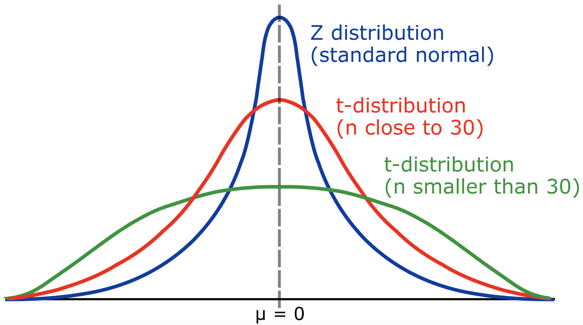
Normal distribution and t-distribution
What are z-tests and t-tests?
z-tests
First, let’s meet its simpler sibling known as z-tests:
z-tests use z-score to measure of how many _standard deviations (std) _below or above the population mean a raw score is.
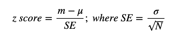
_, N is the sample size, m is the mean of the sample, μ and σ _are the mean and the std of the population respectively.
We use z-scores when there’s a normal distribution (σ and μ are known), and we want to check if the mean of a group is reliably different from that of the population.
Just think z-score is the numbers of std between a value point m (sample mean) and a value point μ (population mean). Note that _SE _in the formula above is the std of the sample distribution, it’s also called the standard error. Go to [1] for SE and sample distribution.
How people came up with the formula?
Here’s the idea. Intuitively, from the population, we will take a vast amount of samples to see if the sample we’re having is likely drawn from that. From the vast samples, we first have a distribution X. Then, we put the sample mean m into X, to see how likely it fits. If m fits so well (we can tell by calculating the z-score to see how far the sample mean to the population mean), we can not deny the Null Hypothesis (H0). Otherwise, we reject H0 because the sample is not likely to be drawn from the population. In other words, in the latter case, we can refuse H0 to accept that the sample is reliably different from the population.
Let’s take a quick look at 2 examples below to understand the idea of z-tests.
Ex1. You have a test score of 190. The test has a mean (μ) of 150 and a standard deviation (σ) of 25. Assume that it’s a normal distribution, your z-score would be?
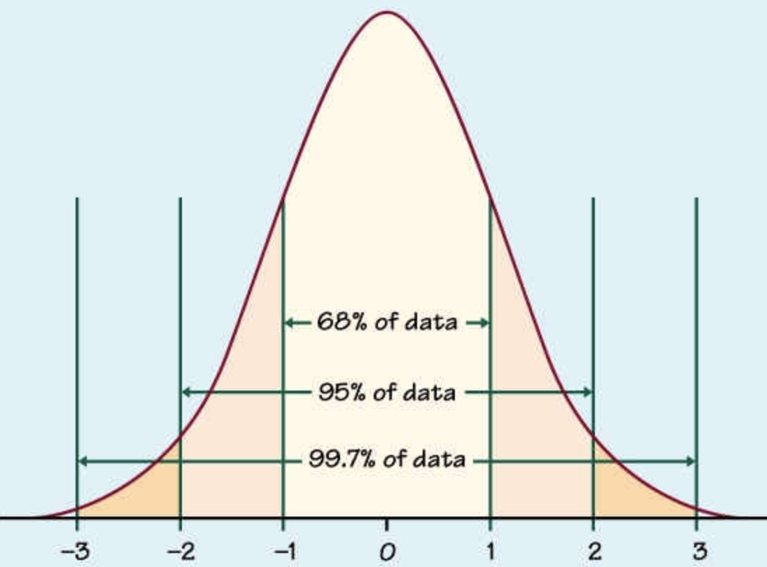
Most of the data lie in +/- 3 std
Ans:
Recall the formula zscore=(m_−_μ)/_SE, _with_ SE_=σ/sqrt(N).
Plug the numbers in:
z-score=(190−150)/ (25/sqrt(1))=1.6
It’s worth noting that in this case, the sample size is 1 because of only your test score in the sample.
Ex2._ In general, the mean height of women is 165 cm with a standard deviation of 5 cm. What is the probability of finding a random sample of 50 women with a mean height of 170 cm, assuming the heights are normally distributed?_
Ans: z-score=(170−165)/(5/sqrt(50)) = 7.07
The sample mean is more than 7 standard deviations from the population mean. Thus, it’s not likely that the sample is from our population. We can safely reject H0.
Any questions so far? If not, here’s a question for you. What happens when N (the sample size) is massive (e.g., 10000)? You can stop here to ponder for a moment before scrolling down.
Ok, we probably have your own answer. The formula can be re-written as (_m_−_μ)*_sqrt(N)/σ_. _At first glance, with a large number _N, _the numerator would be huge as well leading to a large value of _z-score. _Due to the big value of z-score, we reject H0. Something doesn’t sound right here! In fact, if the sample is drawn from the population, so the high chance that its mean (m) is approximately the population mean (μ). So, the numerator should go to 0 (instead of a huge number) which in turn makes z-score so close to 0 no matter how big the denominator is. It now makes sense right? And when the sample is drawn from a totally different population, it’s likely that the more sample you get (i.e., the bigger the sample size is), the easier you can distinguish the sample from the population.
Okay, so far so good. But wait, why on earth we need t-tests when we already have z-tests?
Because of the limitations of the (exact) z-tests.
- Z-tests just work when we know the std of the population (σ). In real life, the std is unknown, hence we have no choice but to estimate std σ from the sample by calculating unbiased sample std (_s) _to perform t-tests. It’s also worth noting that it reminds us of the Chi-squared distribution.
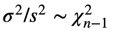
Chi-squared
- If the data is not from a normal distribution, we can not conduct the z-test. Central Limit Theorem might allow us to still make a t-test though.
t-tests
t-tests are parametric procedures consisting of 3 types [2]:
- Two samples T-tests (Independent samples T-test): compare the means of 2 groups to see if they’re reliably different from one another. It’s probably the most popular kind of t-test.
- Paired samples T-tests: test the mean of 1 group twice. Ex: Test balance before and after drinking.
- One sample T-tests: compare the mean of a sample to the mean of the population to see the difference. We’re gonna use this one to solve the watermelon problem.
In general, with O_ne sample t-tests_, we have the same formula as with_ z-tests_, just a little change when the unbiased _sample std _(s) is used to estimate for the std of the population (σ). Because we have to estimate something unknown, we become less confident. Intuitively, the std (i.e., the spread out of data) when we estimate for the population, it has to be greater than the original std calculated from the sample. Instead of divided by _n _to get a “normal” std from the sample, we use n − 1to calculate the _unbiased sample std _(s). The _unbiased sample std _is then used as an approximation for the true std of the population. Mathematically, the degrees of freedom used in this test are n − 1. The less confidence can be expressed as the bell shape of the T-test has heavier tails compared to those of Normal distribution. With more data we have (i.e., the greater the sample size), t-distributions would become more similar to normal distributions.
In terms of Two samples T-test, it’s a bit more tricky. Let’s say we have 2 groups, each has the mean of _m, the varianceof σ², _and the sample size of n. T-score is calculated as formula below.
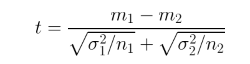
Two samples T-tests
The idea of Two samples T-test is to take the variance between 2 groups, then divided by the variance of each group. In the denominator, n1 and _n2 can be considered normalization factors. _In the figure below, we have 2 same-sized groups with the means of 34, 36, and the std of 6 for both groups. In this case, t-score ~(36–34)/6. Note that we’ve just ignored the normalization factors.
#normal-distribution #statistics #t-test #p-value #hypothesis-testing