Let’s imagine you have data on how long subjects in your study “survived.” Survival could be literal (as in a clinical trial) or figurative (if you are studying customer retention, when people stop reading an article, or when a machine breaks down). In order to visualize the data, we’d like to plot a survival curve, called a Kaplan–Meier curve like the one below.

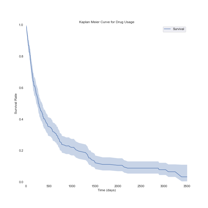
Survival Curve for Drug Tolerance and Usage with 95% confidence interval (artificially generated data, n ≈ 300)

The curve at left (created using artificially generated data) purports to show the percentage of people still taking a medicine some number of days after they start taking it. In this context, they would stop because the medicine was no longer controlling the disease or because it was causing too many side-effects.

Ideally, it would be easy to compute this curve by simply considering the percentage of people who are taking the medicine at a given number of days after they started it.

However, some of the people (about 25% in this example) are still taking the medicine. They may have simply been taking it for a long time (close to 10 years in this case) with no problems or they may have just started it. Such observations are called “right-censored” because we don’t get to observe them later in time (towards the right).

The simplest solution to this is a Kaplan–Meier curve, also called the product–limit estimator. There are other solutions but they require making assumptions about the data and provide a model for it. On the other hand, our usual first step is to just look at the data, and the Kaplan–Meier curve allows us to do that without making assumptions.

In this article we’ll discuss how to compute the Kaplan–Meier curve and, crucially, the confidence intervals displayed. More importantly, we’ll go into the differences between the two ways you could compute the confidence interval (sometimes called ‘log’ and ‘log-log’/exponential Greenwood confidence intervals ).

The Kaplan Meier Estimate

If you haven’t guessed, these sorts of survival curves started in the medical and actuarial worlds where the literal concern was whether someone would in fact die. Consequently, we will adopt the terminology that a given subject in the study (say a person) can either still be alive, in which case the observation is censored (we haven’t observed an event), or they can have died at a particular point in time (we did observe the event).

Note that when we say “time” we don’t mean the literal date, but rather the time relative to when a participant entered the study. In the life-insurance example, that is just when they were born. In the medicine example above, it is when someone starts taking the drug.

#mathematics #time-series-analysis #towards-data-science #data-science #statistics