_You can reach all Python scripts relative to this on my GitHub page. If you are interested, you can also find the scripts used for data cleaning and data visualization for this study in the same repository. And the project is also deployed using Django on Heroku. _View Deployment

Content

1. Data Cleaning (Identifying null values, filling missing values and removing outliers)
2. Data Preprocessing (Standardization or Normalization)
3. ML Models: Linear Regression, Ridge Regression, Lasso, KNN, Random Forest Regressor, Bagging Regressor, Adaboost Regressor, and XGBoost
4. Comparison of the performance of the models
5. Some insights from data

Why is price feature scaled by log transformation?

In the regression model, for any fixed value of X, Y is distributed in this problem data-target value (Price ) not normally distributed, it is right skewed.

To solve this problem, the log transformation on the target variable is applied when it has skewed distribution and we need to apply an inverse function on the predicted values to get the actual predicted target value.

Due to this, for evaluating the model, the RMSLE is calculated to check the error and the R2 Score is also calculated to evaluate the accuracy of the model.

Some Key Concepts:

• **Learning Rate: **Learning rate is a hyper-parameter that controls how much we are adjusting the weights of our network concerning the loss gradient. The lower the value, the slower we travel along the downward slope. While this might be a good idea (using a low learning rate) in terms of making sure that we do not miss any local minima, it could also mean that we’ll be taking a long time to converge — especially if we get stuck on a plateau region.
• n_estimators: This is the number of trees you want to build before taking the maximum voting or averages of predictions. A higher number of trees give you better performance but make your code slower.
• **R² Score: **It is a statistical measure of how close the data are to the fitted regression line. It is also known as the coefficient of determination, or the coefficient of multiple determination for multiple regression. 0% indicates that the model explains none of the variability of the response data around its mean.

1. The Data:

The dataset used in this project was downloaded from Kaggle.

2. Data Cleaning:

The first step is to remove irrelevant/useless features like ‘URL’, ’region_url’, ’vin’, ’image_url’, ’description’, ’county’, ’state’ from the dataset.

As a next step, check missing values for each feature.

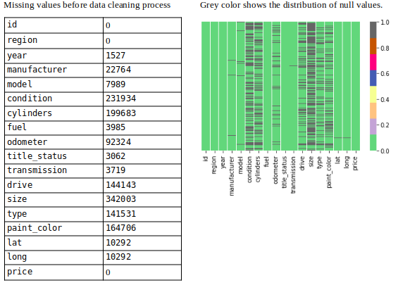
Showing missing values (Image By Panwar Abhash Anil)

Next, now missing values were filled with appropriate values by an appropriate method.

To fill the missing values, IterativeImputer method is used and different estimators are implemented then calculated MSE of each estimator using cross_val_score

1. Mean and Median
2. BayesianRidge Estimator
3. DecisionTreeRegressor Estimator
4. ExtraTreesRegressor Estimator
5. KNeighborsRegressor Estimator

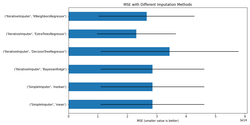
MSE with Different Imputation Methods (Image By Panwar Abhash Anil)

From the above figure, we can conclude that the _ExtraTreesRegressor _estimator will be better for the imputation method to fill the missing value.

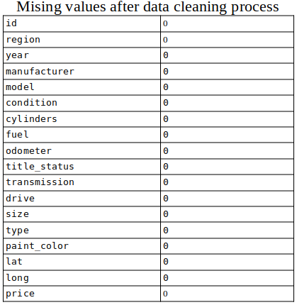
Missing values after filling (Image By Panwar Abhash Anil)

At last, after dealing with missing values there zero null values.

**Outliers: **InterQuartile Range (IQR) method is used to remove the outliers from the data.

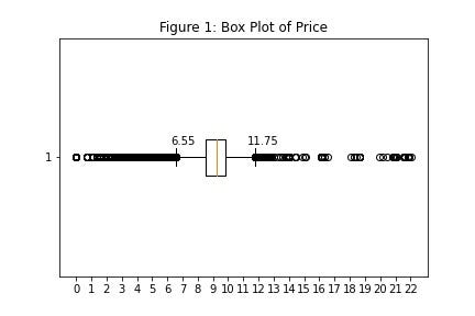
Box Plot of price showing outliers (Image By Panwar Abhash Anil)

Box Plot of Odometer showing outliers (Image By Panwar Abhash Anil)

Box Plot & Histogram of the year (Image By Panwar Abhash Anil)

• From figure 1, the prices whose log is below 6.55 and above 11.55 are the outliers
• From figure 2, it is impossible to conclude something so IQR is calculated to find outliers i.e. odometer values below 6.55 and above 11.55 are the outliers.
• From figure 3, the year below 1995 and above 2020 are the outliers.

At last, Shape of dataset before process= (435849, 25) and after process= (374136, 18). Total 61713 rows and 7 cols removed.

#data-visualization #django #deployment #machine-learning #data-science #deep learning