To evaluate object detection models like R-CNN and YOLO, the mean average precision (mAP) is used. The mAP compares the ground-truth bounding box to the detected box and returns a score. The higher the score, the more accurate the model is in its detections.
In my last article we looked in detail at the confusion matrix, model accuracy, precision, and recall. We used the Scikit-learn library to calculate these metrics as well. Now we’ll extend our discussion to see how precision and recall are used to calculate the mAP.
Here are the sections covered in this tutorial:
- From Prediction Score to Class Label
- Precision-Recall Curve
- Average Precision (AP)
- Intersection over Union (IoU)
- Mean Average Precision (mAP) for Object Detection
Let’s get started.
From Prediction Score to Class Label
In this section we’ll do a quick review of how a class label is derived from a prediction score.
Given that there are two classes, Positive and Negative, here are the ground-truth labels of 10 samples.
y_true = ["positive", "negative", "negative", "positive", "positive", "positive", "negative", "positive", "negative", "positive"]
When these samples are fed to the model it returns the following prediction scores. Based on these scores, how do we classify the samples (i.e. assign a class label to each sample)?
pred_scores = [0.7, 0.3, 0.5, 0.6, 0.55, 0.9, 0.4, 0.2, 0.4, 0.3]
To convert the scores into a class label, a threshold is used. When the score is equal to or above the threshold, the sample is classified as one class. Otherwise, it is classified as the other class. Let’s agree that a sample is Positive if its score is above or equal to the threshold. Otherwise, it is Negative. The next block of code converts the scores into class labels with a threshold of 0.5.
import numpy

pred_scores = [0.7, 0.3, 0.5, 0.6, 0.55, 0.9, 0.4, 0.2, 0.4, 0.3]
y_true = ["positive", "negative", "negative", "positive", "positive", "positive", "negative", "positive", "negative", "positive"]

threshold = 0.5
y_pred = ["positive" if score >= threshold else "negative" for score in pred_scores]
print(y_pred)
['positive', 'negative', 'positive', 'positive', 'positive', 'positive', 'negative', 'negative', 'negative', 'negative']
Now both the ground-truth and predicted labels are available in the y_true and y_pred variables. Based on these labels, the confusion matrix, precision, and recall can be calculated.
r = numpy.flip(sklearn.metrics.confusion_matrix(y_true, y_pred))
print(r)

precision = sklearn.metrics.precision_score(y_true=y_true, y_pred=y_pred, pos_label="positive")
print(precision)

recall = sklearn.metrics.recall_score(y_true=y_true, y_pred=y_pred, pos_label="positive")
print(recall)
## Confusion Matrix (From Left to Right & Top to Bottom: True Positive, False Negative, False Positive, True Negative)
[[4 2]
 [1 3]]

## Precision = 4/(4+1)
0.8

## Recall = 4/(4+2)
0.6666666666666666
After this quick review of calculating the precision and recall, in the next section we’ll discuss creating the precision-recall curve.
Precision-Recall Curve
From the definition of both the precision and recall given in Part 1, remember that the higher the precision, the more confident the model is when it classifies a sample as Positive. The higher the recall, the more positive samples the model correctly classified as Positive.
When a model has high recall but low precision, then the model classifies most of the positive samples correctly but it has many false positives (i.e. classifies many Negative samples as Positive). When a model has high precision but low recall, then the model is accurate when it classifies a sample as Positive but it may classify only some of the positive samples.
Due to the importance of both precision and recall, there is a precision-recall curve the shows the tradeoff between the precision and recall values for different thresholds. This curve helps to select the best threshold to maximize both metrics.
There are some inputs needed to create the precision-recall curve:
- The ground-truth labels.
- The prediction scores of the samples.
- Some thresholds to convert the prediction scores into class labels.
The next block of code creates the y_true list to hold the ground-truth labels, the pred_scores list for the prediction scores, and finally the thresholds list for different threshold values.
import numpy

y_true = ["positive", "negative", "negative", "positive", "positive", "positive", "negative", "positive", "negative", "positive", "positive", "positive", "positive", "negative", "negative", "negative"]

pred_scores = [0.7, 0.3, 0.5, 0.6, 0.55, 0.9, 0.4, 0.2, 0.4, 0.3, 0.7, 0.5, 0.8, 0.2, 0.3, 0.35]

thresholds = numpy.arange(start=0.2, stop=0.7, step=0.05)
Here are the thresholds saved in the thresholds list. Because there are 10 thresholds, 10 values for precision and recall will be created.
[0.2,
 0.25,
 0.3,
 0.35,
 0.4,
 0.45,
 0.5,
 0.55,
 0.6,
 0.65]
The next function named precision_recall_curve() accepts the ground-truth labels, prediction scores, and thresholds. It returns two equal-length lists representing the precision and recall values.
import sklearn.metrics

def precision_recall_curve(y_true, pred_scores, thresholds):
    precisions = []
    recalls = []

    for threshold in thresholds:
        y_pred = ["positive" if score >= threshold else "negative" for score in pred_scores]

        precision = sklearn.metrics.precision_score(y_true=y_true, y_pred=y_pred, pos_label="positive")
        recall = sklearn.metrics.recall_score(y_true=y_true, y_pred=y_pred, pos_label="positive")

        precisions.append(precision)
        recalls.append(recall)

    return precisions, recalls
The next code calls the precision_recall_curve() function after passing the three previously prepared lists. It returns the precisions and recalls lists that hold all the values of the precisions and recalls, respectively.
precisions, recalls = precision_recall_curve(y_true=y_true,
                                             pred_scores=pred_scores,
                                             thresholds=thresholds)
Here are the returned values in the precisions list.
[0.5625,
 0.5714285714285714,
 0.5714285714285714,
 0.6363636363636364,
 0.7,
 0.875,
 0.875,
 1.0,
 1.0,
 1.0]
Here is the list of values in the recalls list.
[1.0,
 0.8888888888888888,
 0.8888888888888888,
 0.7777777777777778,
 0.7777777777777778,
 0.7777777777777778,
 0.7777777777777778,
 0.6666666666666666,
 0.5555555555555556,
 0.4444444444444444]
Given the two lists of equal lengths, it is possible to plot their values in a 2D plot as shown below.
matplotlib.pyplot.plot(recalls, precisions, linewidth=4, color="red")
matplotlib.pyplot.xlabel("Recall", fontsize=12, fontweight='bold')
matplotlib.pyplot.ylabel("Precision", fontsize=12, fontweight='bold')
matplotlib.pyplot.title("Precision-Recall Curve", fontsize=15, fontweight="bold")
matplotlib.pyplot.show()
The precision-recall curve is shown in the next figure. Note that as the recall increases, the precision decreases. The reason is that when the number of positive samples increases (high recall), the accuracy of classifying each sample correctly decreases (low precision). This is expected, as the model is more likely to fail when there are many samples.
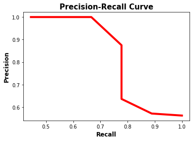
The precision-recall curve makes it easy to decide the point where both the precision and recall are high. According to the previous figure, the best point is (recall, precision)=(0.778, 0.875).
Graphically deciding the best values for both the precision and recall might work using the previous figure because the curve is not complex. A better way is to use a metric called the f1 score, which is calculated according to the next equation.
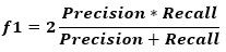
The f1 metric measures the balance between precision and recall. When the value of f1 is high, this means both the precision and recall are high. A lower f1 score means a greater imbalance between precision and recall.
According to the previous example, the f1 is calculated according to the code below. According to the values in the f1 list, the highest score is 0.82352941. It is the 6th element in the list (i.e. index 5). The 6th elements in the recalls and precisions lists are 0.778 and 0.875, respectively. The corresponding threshold value is 0.45.
f1 = 2 * ((numpy.array(precisions) * numpy.array(recalls)) / (numpy.array(precisions) + numpy.array(recalls)))
[0.72,
 0.69565217,
 0.69565217,
 0.7,
 0.73684211,
 0.82352941,
 0.82352941,
 0.8,
 0.71428571, 0
 .61538462]
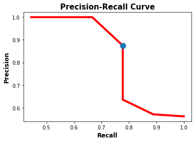
The next figure shows, in blue, the location of the point that corresponds to the best balance between the recall and the precision. In conclusion, the best threshold to balance the precision and recall is 0.45 at which the precision is 0.875 and the recall is 0.778.
matplotlib.pyplot.plot(recalls, precisions, linewidth=4, color="red", zorder=0)
matplotlib.pyplot.scatter(recalls[5], precisions[5], zorder=1, linewidth=6)

matplotlib.pyplot.xlabel("Recall", fontsize=12, fontweight='bold')
matplotlib.pyplot.ylabel("Precision", fontsize=12, fontweight='bold')
matplotlib.pyplot.title("Precision-Recall Curve", fontsize=15, fontweight="bold")
matplotlib.pyplot.show()
After the precision-recall curve is discussed, the next section discusses how to calculate the average precision.
#deep-learning #data-science #developer