It is easy for us to visualize two or three dimensional data, but once it goes beyond three dimensions, it becomes much harder to see what high dimensional data looks like.
Today we are often in a situation that we need to analyze and find patterns on datasets with thousands or even millions of dimensions, which makes visualization a bit of a challenge. However, a tool that can definitely help us better understand the data is dimensionality reduction.
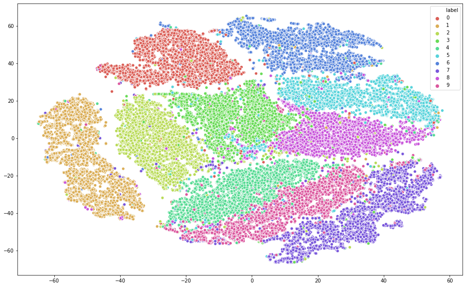
In this post, I will discuss t-SNE, a popular non-linear dimensionality reduction technique and how to implement it in Python using sklearn. The dataset I have chosen here is the popular MNIST dataset.
Table of Curiosities
- What is t-SNE and how does it work?
- How is t-SNE different with PCA?
- How can we improve upon t-SNE?
- What are the limitations?
- What can we do next?
Overview
T-Distributed Stochastic Neighbor Embedding, or t-SNE, is a machine learning algorithm and it is often used to embedding high dimensional data in a low dimensional space [1].
In simple terms, the approach of t-SNE can be broken down into two steps. The first step is to represent the high dimensional data by constructing a probability distribution P, where the probability of similar points being picked is high, whereas the probability of dissimilar points being picked is low. The second step is to create a low dimensional space with another probability distribution Q that preserves the property of P as close as possible.
In step 1, we compute the similarity between two data points using a conditional probability p. For example, the conditional probability of j given i represents that x_j would be picked by x_i as its neighbor assuming neighbors are picked in proportion to their probability density under a Gaussian distribution centered at _x_i _[1]. In step 2, we let _y_i _and y_j to be the low dimensional counterparts of x_i and _x_j, _respectively. Then we consider q to be a similar conditional probability for y_j being picked by y_i and we employ a **student t-distribution **in the low dimension map. The locations of the low dimensional data points are determined by minimizing the Kullback–Leibler divergence of probability distribution P from Q.
#data-visualization #sklearn #dimensionality-reduction #data-science #machine-learning #data analysis