Optimization Algorithms in Deep Learning
In this article, I will present to you the most sophisticated optimization algorithms in Deep Learning that allow neural networks to learn faster and achieve better performance.
These algorithms are Stochastic Gradient Descent with Momentum, AdaGrad, RMSProp, and Adam Optimizer.
Table of Content
- Why do we need better optimization Algorithms?
- Stochastic Gradient Descent with Momentum
- AdaGrad
- RMSProp
- Adam Optimizer
- What is the best Optimization Algorithm for Deep Learning?
1. Why do we need better optimization Algorithms?
To train a neural network model, we must define a loss function in order to measure the difference between our model predictions and the label that we want to predict. What we are looking for is a certain set of weights, with which the neural network can make an accurate prediction, which automatically leads to a lower value of the loss function.
I think you must know by now, that the mathematical method behind it is called gradient descent.
Eq. 1 Gradient Descent for parameters θ with loss function L.
In this technique (Eq.1), we must calculate the gradient of the loss function L with respect to the weights (or parameters θ) that we want to improve. Subsequently, the weights/parameters are updated in the direction of the negative direction of the gradient.
By periodically applying the gradient descent to the weights, we will eventually arrive at the optimal weights that minimize the loss function and allow the neural network to make better predictions.
So far the theory.
Do not get me wrong, gradient descent is still a powerful technique. In practice, however, this technique may encounter certain problems during training that can slow down the learning process or, in the worst case, even prevent the algorithm from finding the optimal weights
These problems were on the one hand saddle points and local minima of the loss function, where the loss function becomes flat and the gradient goes to zero:

Fig. 1 Saddle Points and Local Minima
A gradient near zero does not improve the weight parameters and prevents the entire learning process.
On the other hand, even if we have gradients that are not close to zero, the values of these gradients calculated for different data samples from the training set may vary in value and direction. We say that the gradients are noisy or have a lot of variances. This leads to a zigzag movement towards the optimal weights and can make learning much slower:
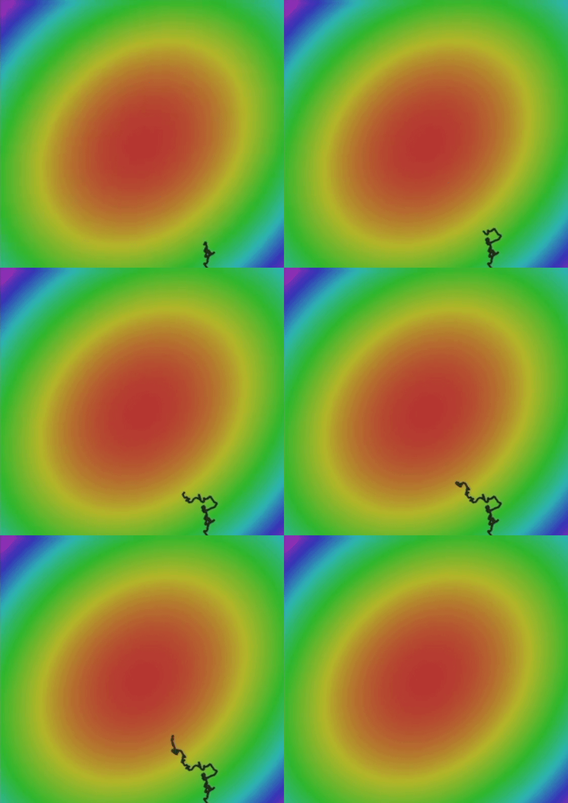
Fig. 3 Example of zig-zag movements of noisy gradients.
In the following article, we are going to learn about more sophisticated gradient descent algorithms. All of these algorithms are based on the regular gradient descent optimization that we have come to know so far. But we can extend this regular approach for the weight optimization by some mathematical tricks to build even more effective optimization algorithms that allow our neural network to adequately handle these problems, thereby learning faster and to achieve a better performance
2. Stochastic Gradient Descent with Momentum
The first of the sophisticated algorithms I want to present you is called stochastic gradient descent with momentum.

Eq. 2 Equations for stochastic gradient descent with momentum.
On the left side in Eq. 2, you can see the equation for the weight updates according to the regular stochastic stochastic gradient descent. The equation on the right shows the rule for the weight updates according to the SGD with momentum. The momentum appears as an additional term ρ times v that is added to the regular update rule.
Intuitively speaking, by adding this momentum term we let our gradient to build up a kind of velocity v during training. The velocity is the running sum of gradients weighted by ρ.
ρ can be considered as friction that slows down the velocity a little bit. In general, you can see that the velocity builds up over time. By using the momentum term saddle points and local minima become less dangerous for the gradient. Because step sizes towards the global minimum now don’t depend only on the gradient of the loss function at the current point, but also on the velocity that has built up over time.
In other words, we are moving more towards the direction of velocity than towards the gradient at a certain point.
If you want to have a physical representation of the stochastic gradient descent with momentum think about a ball that rolls down a hill and builds up velocity over time. If this ball reaches some obstacles on its way, such as a hole or a flat ground with no downward slope, the velocity v would give the ball enough power to roll over these obstacles. In this case, the flat ground and the hole represent saddle points or local minima of a loss function.
In the following video (Fig. 4), I want to show you a direct comparison of regular stochastic gradient descent and stochastic gradient descent with momentum term. Both algorithms are trying to reach the global minimum of the loss function which lives in a 3D space. Please note how the momentum term makes the gradients to have less variance and fewer zig-zags movements.

Fig. 4 SGD vs. SGD with Momentum
In general, the momentum term makes converges towards optimal weights more stable and faster.
3. AdaGrad
Another optimization strategy is called AdaGrad. The idea is that you keep the running sum of squared gradients during optimization. In this case, we have no momentum term, but an expression g that is the sum of the squared gradients.

Eq. 3 Parameter update rule for AdaGrad.
When we update a weight parameter, we divide the current gradient by the root of that term g. To explain the intuition behind AdaGrad, imagine a loss function in a two-dimensional space in which the gradient of the loss function in one direction is very small and very high in the other direction.
Summing up the gradients along the axis where the gradients are small causes the squared sum of these gradients to become even smaller. If during the update step, we divide the current gradient by a very small sum of squared gradients g, the result of that division becomes very high and vice versa for the other axis with high gradient values.
As a result, we force the algorithm to make updates in any direction with the same proportions.
This means that we accelerate the update process along the axis with small gradients by increasing the gradient along that axis. On the other hand, the updates along the axis with the large gradient slow down a bit.
However, there is a problem with this optimization algorithm. Imagine what would happen to the sum of the squared gradients when training takes a long time. Over time, this term would get bigger. If the current gradient is divided by this large number, the update step for the weights becomes very small. It is as if we were using very low learning that becomes even lower the longer the training goes. In the worst case, we would get stuck with AdaGrad and the training would go on forever.
4. RMSProp
There is a slight variation of AdaGrad called RMSProp that addresses the problem that AdaGrad has. With RMSProp we still keep the running sum of squared gradients but instead of letting that sum grow continuously over the period of training we let that sum actually decay.
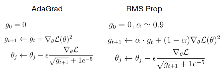
Eq. 4 Update rule for RMS Prop.
In RMSProp we multiply the sum of squared gradients by a decay rate α and add the current gradient weighted by (1- α). The update step in the case of RMSProp looks exactly the same as in AdaGrad where we divide the current gradient by the sum of squared gradients to have this nice property of accelerating the movement along the one dimension and slowing down the movement along the other dimension.
Let’s see how RMSProp is doing in comparison with SGD and SGD with momentum in finding the optimal weights.

Fig. 5 SGD vs. SGD with Momentum vs. RMS Prop
Although SGD with momentum is able to find the global minimum faster, this algorithm takes a much longer path, that could be dangerous. Because a longer path means more possible saddle points and local minima. RMSProp, on the other hand, goes straight towards the global minimum of the loss function without taking a detour.
5. Adam Optimizer
So far we have used the moment term to build up the velocity of the gradient to update the weight parameter towards the direction of that velocity. In the case of AdaGrad and RMSProp, we used the sum of the squared gradients to scale the current gradient, so we could do weight updates with the same ratio in each dimension.
These two methods seemed pretty good ideas. Why do not we just take the best of both worlds and combine these ideas into a single algorithm?
This is the exact concept behind the final optimization algorithm called Adam, which I would like to introduce to you.
The main part of the algorithm consists of the following three equations. These equations may seem overwhelming at first, but if you look closely, you’ll see some familiarity with previous optimization algorithms.
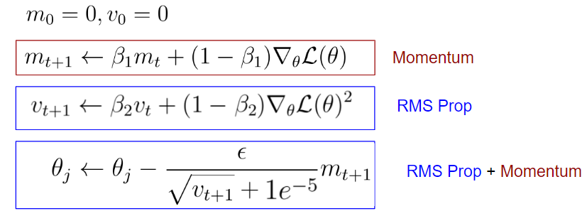
Eq. 5 Parameter update rule for Adam Optimizer
The first equation looks a bit like the SGD with momentum. In the case, the term would be the velocity and the friction term. In the case of Adam, we call the first momentum and is just a hyperparameter.
The difference to SGD with momentum, however, is the factor (1- β1), which is multiplied with the current gradient.
The second part of the equations, on the other hand, can be regarded as RMSProp, in which we are keeping the running sum of squared gradients. Also, in this case, there is the factor (1-β2) which is multiplied with the squared gradient.
The term in the equation is called the second momentum and is also just a hyperparameter. The final update equation can be seen as a combination of RMSProp and SGD with Momentum.
So far, Adam has integrated the nice features of the two previous optimization algorithms, but here’s a little problem, and that’s the question of what happens in the beginning.
At the very first time step, the first and second momentum terms are initialized to zero. After the first update of the second momentum, this term is still very close to zero. When we update the weight parameters in the last equation, we divide by a very small second momentum term v, resulting in a very large first update step.
This first very large update step is not the result of the geometry of the problem, but it is an artifact of the fact that we have initialized the first and second momentum to zero. To solve the problems of large first update steps, Adam includes a correction clause:
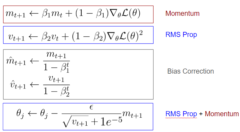
Eq. 6 Bias Correction for Adam Optimizer
You can see that after the first update of the first and second momentum and we make an unbiased estimate of these momentums by taking into account the current time step. These correction terms make the values of the first and second momentum to be higher in the beginning than in the case without the bias correction.
As a result, the first update step of the neural network parameters does not get that large and we don’t mess up our training in the beginning. The additional bias corrections give us the full form of Adam Optimizer.
Now, let us compare all algorithms with each other in terms of finding the global minimum of the loss function:

Fig. 6 Comparison of all optimization algorithms.
6. What is the best Optimization Algorithm for Deep Learning?
Finally, we can discuss the question of what the best gradient descent algorithm is.
In general, a normal gradient descent algorithm is more than adequate for simpler tasks. If you are not satisfied with the accuracy of your model you can try out RMSprop or add a momentum term to your gradient descent algorithms.
But in my experience the best optimization algorithm for neural networks out there is Adam. This optimization algorithm works very well for almost any deep learning problem you will ever encounter. Especially if you set the hyperparameters to the following values:
- β1=0.9
- β2=0.999
- Learning rate = 0.001–0.0001
… this would be a very good starting point for any problem and virtually every type of neural network architecture I’ve ever worked with.
That’s why Adam Optimizer is my default optimization algorithm for every problem I want to solve. Only in very few cases do I switch to other optimization algorithms that I introduced earlier.
In this sense, I recommend that you always start with the Adam Optimizer, regardless of the architecture of the neural network of the problem domain you are dealing with.
#deep-learning #machine-learning #data-science
