A crash course on the Beta distribution, binomial likelihood, and conjugate priors for A/B testing

Frequentist background

If you’re anything like me, long before you were interested in data science, machine learning, etc, you gained your initial exposure to statistics through the social sciences. In domains such as psychology, sociology, etc, a study is often conducted over a period of time (that might be days, months, or even years.) In the case of novel experiments, the results are collected, maximum likelihood estimates are produced for the mean and variance, and confidence intervals are constructed.

Alternatively, if we hypothesize that things don’t function as described by the incumbent model (aka null hypothesis), we reference the existing data, examine the mean, variance, and confidence interval, collect data via a study (sample from the population) and compare our sample mean to the confidence interval. If the sample mean is extreme, we reject the null hypothesis and conclude, “the incumbent model’s mean and variance are inaccurate, more study is required. Or we simply fail to reject_ the incumbent model’s findings. What does extreme mean? It’s a bit subjective — it means that the finding was highly improbable according to the incumbent model’s distribution and an arbitrary threshold. (ie given the distribution, our sample would have only been observed to be so large (or larger) or so small (or smaller) 1% of the time and we arbitrarily decided that we would reject the incumbent model if such a finding had a 5% chance of occurrence (or an even lesser probability.)

This is the frequentist paradigm. It’s well-suited for situations where we have the luxury of waiting a long period of time to collect enough data to be pretty sure about the shape and central tendencies of our population of interest before acting on our understanding. Unfortunately, this approach is ill-suited for situations where we are short on resources (time and data) and need to make the best decision given what we presently know.

Enter Bayesian statistics!

Before we jump into Bayesian statistics, let’s recap some key elements of the frequentist paradigm. the parameters that govern a distribution are fixed we simply need to collect a big enough sample for our estimates (sample statistics) to converge on the true population parameters. Given that our parameters are inherently scalar values (fixed numbers), we articulate our confidence in these values through confidence intervals (in other words, in terms of how probable an observation would be under the current parameters’ MLE estimates.)

The Bayesian model rejects the idea that parameters are fixed and views them as distributions, themselves. This makes the math much, much less pleasant. However, it allows us to start with a belief about the parameter (prior), relate this belief to the data observed (likelihood), itself, consider all other possibilities (evidence), and returns new updated beliefs (posterior.) In other words, it’s optimized for online learning and one such widely applicable example of online learning is A/B testing.

Before we can jump into coding, let’s talk strategy — if you’ve googled Bayesian Statistics before, you’ve likely heard of terms like Markov Chain Monte Carlo (MCMC methods). These methods were invented to sample from distributions that are extremely difficult ( if not impossible ) to integrate analytically and they’re largely oriented about the evidence See section 4 below on Bayes Rule.

Bayes Rule summed up is (A) pick a prior distribution; it’s your pre-inference beliefs about the parameter of interest. Then (B) choose a likelihood to model how surprising (or unsurprising) the data is, conditioned on the prior belief. And finally, © compare the numerator to the evidence. This is literally, the probability of observing the data under any _value _that the parameter could take on. The evidence evaluates to a constant value, which scales the numerator, such that it’s a valid probability distribution (integrates to 1.)

In reality, the more complex your model, the more painful computing the evidence will become. Enter conjugate priors. There are certain combinations of priors and likelihoods, which are “conjugate to one another” if the posterior (your updated beliefs about the parameter)** takes the same shape as the prior (and is generally, easy to compute!)

In this article, we will exploit a conjugate prior in order to reduce computational complexity! One such perfect example is the Beta prior, Binomial likelihood pairing — where the posterior distribution is also described by the Beta distribution.

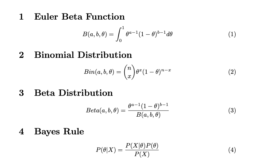
First things first, the Euler Beta Function is not the same as the Beta distribution; you will save yourself substantial confusion by committing this to memory now. See section 1 below. In fact, the Euler Beta Function is the denominator of the Beta Distribution (see section 3.) Its purpose is to scale the numerator such that the Beta distribution integrates to 1 (common theme)

The Binomial Distribution describes a summation of Bernoulli trials. Theta is raised to the x power (how many successes) and multiplied by one minus theta raised to the n minus x power (failures in n trials.) The first term, read “n choose x” is the number of combinations (regardless of order) in which x total successes could occur in n trials. For our A/B test, we could be talking about any binary success/failure (slot machines conversions vs total website hits, etc) it’s a reasonable likelihood choice.

I warned you the evidence was very, very nasty didn’t I? See section 4.3 below. Of note, our strategy relies on factoring constants out of the integral, namely, n-Choose-x divided by the the Euler Beta Function. After this, we can combine like terms easily, arriving at what looks very similar to another Euler Beta Function (the exponent values have changed, but this will prove to be beneficial.)

#towards-data-science #statistics #machine-learning #data-science #python #testing