Multi-Label Image Classification in TensorFlow 2.0

Do you want to build amazing things with AI? There are many things you could learn. The newly released TensorFlow 2.0 has made deep learning development much easier by integrating more high level APIs. If you are already an ML practioner and still did not join the TF world, you have no excuse anymore! The entry ticket is almost free.

In this blog post, I will describe some concepts and tools that you could find interesting when training multi-label image classifiers.

Table of contents

• Understand multi-label classification
• What is interesting in TensorFlow 2.0
• The dataset (Movie Genre from its Poster)
• Build a fast input pipeline
• Transfer learning with TF.Hub
• Model training and evaluation
• Export Keras model

Understand multi-label classification

Machine learning has showed tremendous success these recent years in solving complex prediction tasks at a scale that we couldn’t imagine before. The easiest way to start transforming a business with it, is to identify simple binary classification tasks, acquire a sufficient amount of historical data and train a good classifier to generalize well in the real world. There is always some way to frame a predictive business question into a Yes/No question. Is a customer going to churn? Will an ad impression generate a click? Will a click generate a conversion? All these binary questions can be addressed with supervised learning if you collect labeled data.

We can also design more complex supervised learning systems to solve non-binary classification tasks:

• Multi-class classification: There are more than two classes and every observation belongs to one and only one class. E.g., An ecommerce company wants to categorize products like smartphones based on their brands (Samsung, Huawei, Apple, Xiaomi, Sony or Other).
• Multi-label classification: There are two classes or more and every observation belongs to one or multiple classes at the same time. Example of application is medical diagnosis where we need to prescribe one or many treatments to a patient based on his signs and symptoms.
  By analogy, we can design a multi-label classifier for car diagnosis. It takes as input all electronic measures, errors, symptoms, mileage and predicts the parts that need to be replaced in case of incident on the car.

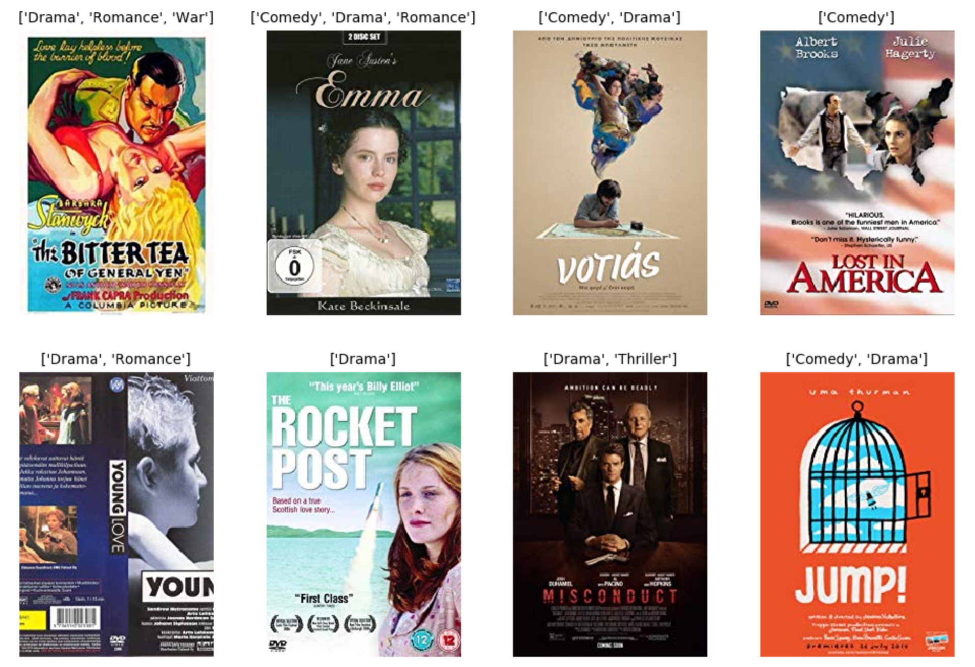
Multi-label classification is also very common in computer vision applications. We, humans, use our instinct and impressions to guess the content of a new movie when seing its poster (action? drama? comedy? etc.). You have probably been in such situation in a metro station where you wanted to guess the genre of a movie from a wall poster. If we assume that in your inference process, you are using the color information of the poster, saturation, hues, texture of the image, body or facial expression of the actors and any shape or design that makes a genre recognizable, then maybe there is a numerical way to extract those significant patterns from the poster and learn from them in a similar manner. How to build a deep learning model that learns to predict movie genres? Let’s see some techniques you can use in TensorFlow 2.0!

What is interesting in TensorFlow 2.0

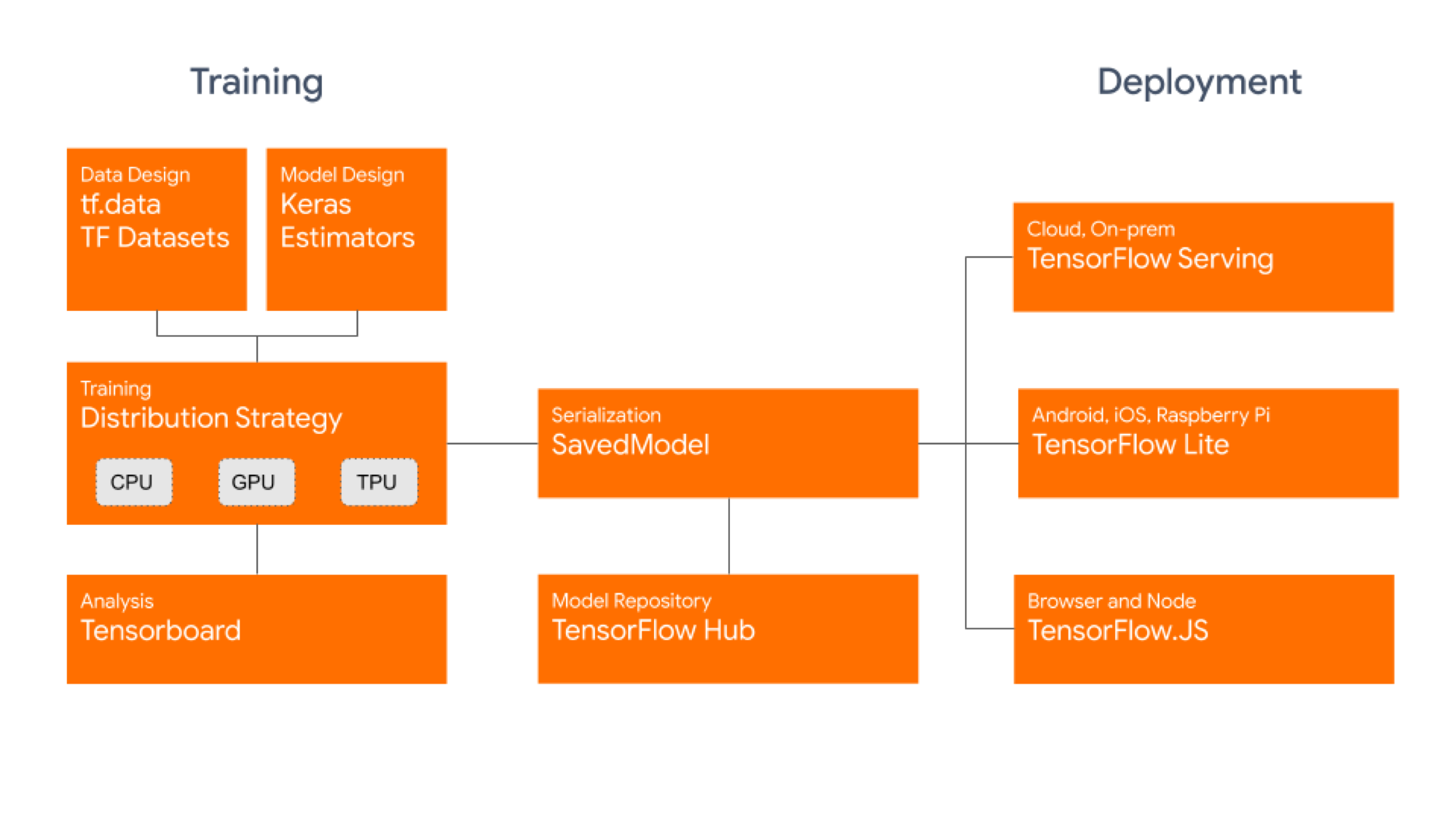
When TensorFlow was first released by Google in 2015, it rapidly became the world’s most popular open-source machine learning library — “a comprehensive ecosystem of tools for developers, enterprises, and researchers who want to push the state-of-the-art in machine learning and build scalable ML-powered applications.” Google annouced the official release of TensorFlow 2.0 by the end of September this year. The new version adds major features and improvements:

• Full integration of Keras with eager execution by default
• More Pythonic function execution with tf.function which makes TensorFlow graphs well optimized for parallel computation
• Faster input pipelines with TensorFlow Datasets for passing in training and validation data in a very efficient way
• More robust deployment in production on servers, devices and web browsers with TensorFlow Serving, TensorFlow Lite and TensorFlow.js

Personaly, I enjoyed building custom estimators in TensorFlow 1.x because they provide a high level of flexibility. So, I was happy to see the Estimator API being extended. We can now create estimators by converting existing Keras models.

The dataset (Movie Genre from its Poster)

This dataset is hosted on Kaggle and contains movie posters from IMDB Website. A csv fileMovieGenre.csv can be downloaded. It contains the following information for each movie: IMDB Id, IMDB Link, Title, IMDB Score, Genre and a link to download the movie poster. In this dataset, each Movie poster can belong to at least one genre and can have at most 3 labels assigned to it. The total number of posters is around 40K.

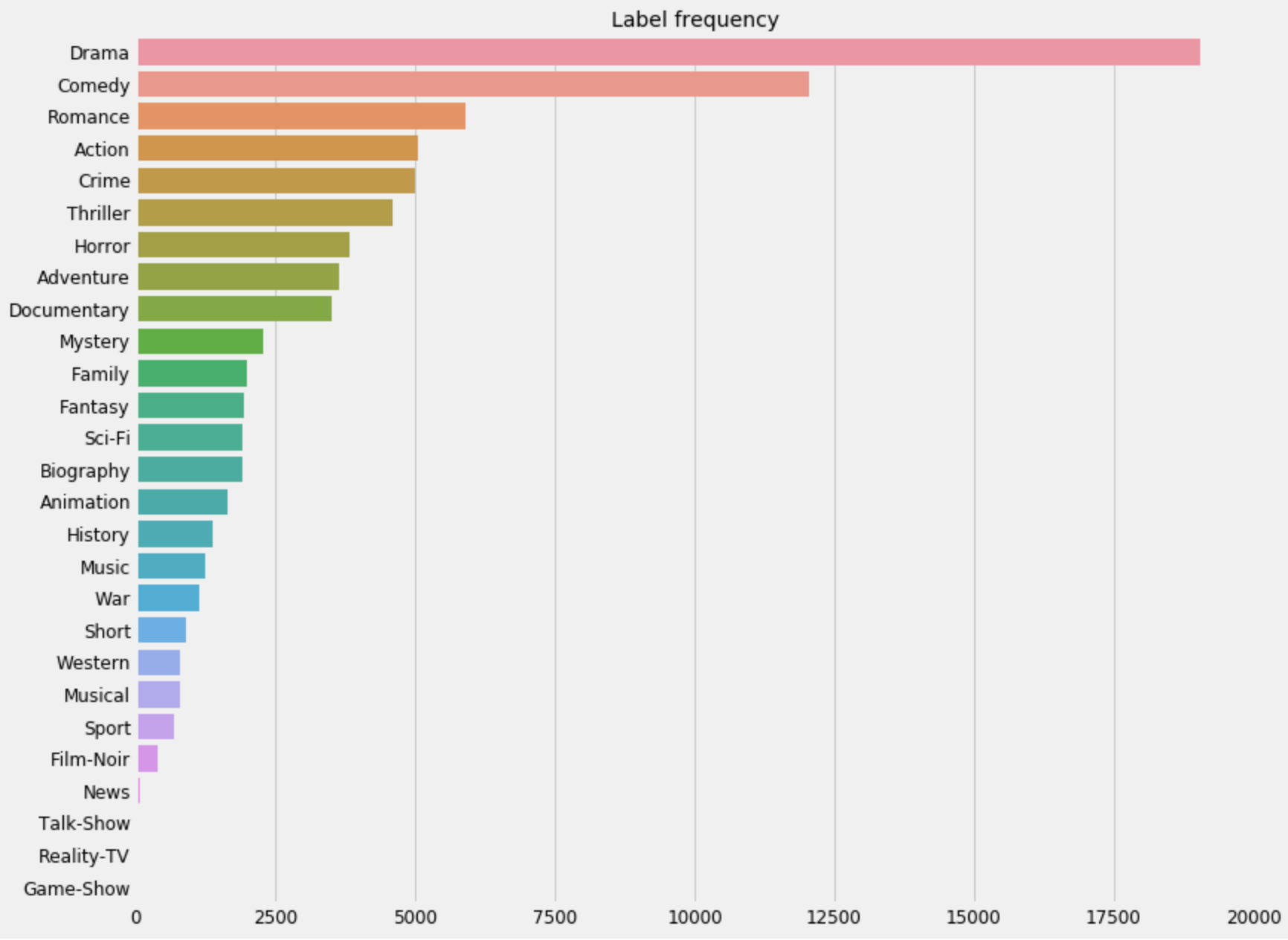
Something important to notice is that all movie genres are not represented in the same quantity. Some of them can be very infrequent which may represent a hard challenge for any ML algorithm. You can decide to ignore all labels with less than 1000 observations (Short, Western, Musical, Sport, Film-Noir, News, Talk-Show, Reality-TV, Game-Show). This means that the model will not be trained to predict those labels due to the lack of observations on them.

Build a fast input pipeline

If you are familiar with keras.preprocessing you may know the image data iterators (E.g., ImageDataGenerator, DirectoryIterator). These iterators are convenient for multi-class classfication where the image directory contains one subdirectory for each class. But, in the case of multi-label classification, having an image directory that respects this structure is not possible because one observation can belong to multiple classes at the same time.

That is where the tf.data API has the upper hand.

• It is faster
• It provides fine-grained control
• It is well integrated with the rest of TensorFlow

You first need to write some function to parse image files and generate a tensor representing the features and a tensor representing the labels.

• In the parsing function you can resize the image to adapt to the input expected by the model.
• You can also scale the pixel values to be between 0 and 1. This is a common practice that helps speed up the convergence of training. If you consider every pixel as a feature, you would like these features to have a similar range so that the gradients don’t go out of control and that you only need one global learning rate multiplier.

IMG_SIZE = 224 # Specify height and width of image to match the input format of the modelCHANNELS = 3 # Keep RGB color channels to match the input format of the model

IMG_SIZE = 224 # Specify height and width of image to match the input format of the model

CHANNELS = 3 # Keep RGB color channels to match the input format of the model

def parse_function(filename, label):
    """Function that returns a tuple of normalized image array and labels array.
    Args:
        filename: string representing path to image
        label: 0/1 one-dimensional array of size N_LABELS
    """
    # Read an image from a file
    image_string = tf.io.read_file(filename)
    # Decode it into a dense vector
    image_decoded = tf.image.decode_jpeg(image_string, channels=CHANNELS)
    # Resize it to fixed shape
    image_resized = tf.image.resize(image_decoded, [IMG_SIZE, IMG_SIZE])
    # Normalize it from [0, 255] to [0.0, 1.0]
    image_normalized = image_resized / 255.0
    return image_normalized, label

To train a model on our dataset you want the data to be:

• Well shuffled
• Batched
• Batches to be available as soon as possible.

These features can be easily added using the tf.data.Dataset abstraction.

BATCH_SIZE = 256 # Big enough to measure an F1-score

AUTOTUNE = tf.data.experimental. AUTOTUNE # Adapt preprocessing and prefetching dynamically to reduce GPU and CPU idle time

SHUFFLE_BUFFER_SIZE = 1024 # Shuffle the training data by a chunck of 1024 observations

AUTOTUNE will adapt the preprocessing and prefetching workload to model training and batch consumption. The number of elements to prefetch should be equal to (or possibly greater than) the number of batches consumed by a single training step. AUTOTUNE will prompt the tf.data runtime to tune the value dynamically at runtime.

You can now create a function that generates training and validation datasets for TensorFlow.

def create_dataset(filenames, labels, is_training=True):
    """Load and parse dataset.
    Args:
        filenames: list of image paths
        labels: numpy array of shape (BATCH_SIZE, N_LABELS)
        is_training: boolean to indicate training mode
    """
    
    # Create a first dataset of file paths and labels
    dataset = tf.data.Dataset.from_tensor_slices((filenames, labels))
    # Parse and preprocess observations in parallel
    dataset = dataset.map(parse_function, num_parallel_calls=AUTOTUNE)
    
    if is_training == True:
        # This is a small dataset, only load it once, and keep it in memory.
        dataset = dataset.cache()
        # Shuffle the data each buffer size
        dataset = dataset.shuffle(buffer_size=SHUFFLE_BUFFER_SIZE)
        
    # Batch the data for multiple steps
    dataset = dataset.batch(BATCH_SIZE)
    # Fetch batches in the background while the model is training.
    dataset = dataset.prefetch(buffer_size=AUTOTUNE)
    
    return dataset

train_ds = create_dataset(X_train, y_train_bin)
val_ds = create_dataset(X_val, y_val_bin)

Each batch will be a pair of arrays (one that holds the features and another one that holds the labels). The features array will be of shape (BATCH_SIZE, IMG_SIZE, IMG_SIZE, CHANNELS) containing the scaled pixels. The labels array will be of shape (BATCH_SIZE, N_LABELS) where N_LABELS is the maximum number of target labels and each value represents wether a movie has a particular genre in it (0 or 1 value).

Transfer learning with TF.Hub

Instead of building and training a new model from scratch, you can use a pre-trained model in a process called transfer learning. The majority of pre-trained models for vision applications were trained on ImageNet which is a large image database with more than 14 million images divided into more than 20 thousand categories. The idea behind transfer learning is that these models, because they were trained in a context of large and general classification tasks, can then be used to address a more specific task by extracting and transfering meaningful features that were previously learned. All you need to do is acquire a pre-trained model and simply add a new classfier on top of it. The new classification head will be trained from scratch so that you repurpose the objective to your multi-label classfication task.

Aknowledgement
TensorFlow core team did a great job sharing pre-trained models and tutorials on how to use them with tf.keras API.
transfer learning with hub
transfer learning by François Chollet

What is TensorFlow Hub?

One concept that is essential in software development is the idea of reusing code that is made available through libraries. Libraries make the development faster and generate more efficiency. For machine learning engineers working on computer vision or NLP tasks, we know how long it takes to train complex neural network architectures from scratch. TensorFlow Hub is a library that allows to publish and reuse pre-made ML components. Using TF.Hub, it becomes simple to retrain the top layer of a pre-trained model to recognize the classes in a new dataset. TensorFlow Hub also distributes models without the top classification layer. These can be used to easily perform transfer learning.

Download a headless model

Any Tensorflow 2 compatible image feature vector URL from tfhub.dev can be interesting for our dataset. The only condition is to insure that the shape of image features in our prepared dataset matches the expected input shape of the model you want to reuse.

First, let’s prepare the feature extractor. We will be using a pre-trained instance of MobileNet V2 with a depth multiplier of 1.0 and an input size of 224x224. MobileNet V2 is actually a large family of neural network architectures that were mainly designed to speed up on-device inference. They come in different sizes depending on the depth multiplier (number of features in hidden convolutional layers) and the size of input images.

import tensorflow_hub as hub

feature_extractor_url = "https://tfhub.dev/google/imagenet/mobilenet_v2_100_224/feature_vector/4"
feature_extractor_layer = hub.KerasLayer(feature_extractor_url,
                                         input_shape=(IMG_SIZE,IMG_SIZE,CHANNELS))

The feature extractor we are using here accepts images of shape (224, 224, 3) and returns a 1280-length vector for each image.

You should freeze the variables in the feature extractor layer, so that the training only modifies the new classification layers. Usually, it is a good practice when working with datasets that are very small compared to the orginal dataset the feature extractor was trained on.

feature_extractor_layer.trainable = False

Fine tuning the feature extractor is only recommended if the training dataset is large and very similar to the original ImageNet dataset.

Attach a classification head

Now, you can wrap the feature extractor layer in a tf.keras.Sequential model and add new layers on top.

model = tf.keras.Sequential([
    feature_extractor_layer,
    layers.Dense(1024, activation='relu', name='hidden_layer'),
    layers.Dense(N_LABELS, activation='sigmoid', name='output')
])

Here is what the model summary looks like:

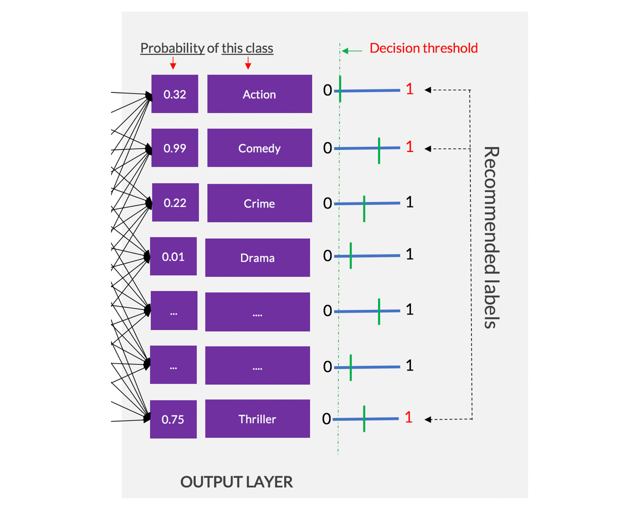
The 2.2M parameters in MobileNet are frozen, but there are 1.3K trainable parameters in the dense layers. You need to apply the sigmoid activation function in the final neurons to ouput a probability score for each genre apart. By doing so, you are relying on multiple logistic regressions to train simultaneously inside the same model. Every final neuron will act as a seperate binary classifier for one single class, even though the features extracted are common to all final neurons.

When generating predictions with this model, you should expect an independant probability score for each genre and that all probability scores do not necessarily sum up to 1. This is different from using a softmax layer in multi-class classification where the sum of probability scores in the output is equal to 1.

Model training and evaluation

After preparing the dataset and composing a model by attaching a multi-label neural network classifier on top of a pre-trained model, you can proceed to training and evaluation but first you need to define two major functions:

• A loss function: You need it to measure the model error (cost) on traning batches. It has to be differentiable in order to backpropagate the error in the neural network and update the weights.
• An evaluation function: It should represent the final evaluation metric you really care about. Unlike the loss function it has to be more intuitive in order to understand the performance of the model in the real world.

Suppose you want to use the Macro F1-score @ threshold 0.5 to evaluate the performance of the model. It is the average of all F1-scores obtained when fixing a probability threshold of 0.5 for each label. Taking the average over all labels is very reasonable if they have the same importance in the multi-label classification task. I am providing here an implementation of this metric on a batch of observations in TensorFlow.

def macro_f1(y, y_hat, thresh=0.5):
    """Compute the macro F1-score on a batch of observations (average F1 across labels)
    
    Args:
        y (int32 Tensor): labels array of shape (BATCH_SIZE, N_LABELS)
        y_hat (float32 Tensor): probability matrix from forward propagation of shape (BATCH_SIZE, N_LABELS)
        thresh: probability value above which we predict positive
        
    Returns:
        macro_f1 (scalar Tensor): value of macro F1 for the batch
    """
    y_pred = tf.cast(tf.greater(y_hat, thresh), tf.float32)
    tp = tf.cast(tf.math.count_nonzero(y_pred * y, axis=0), tf.float32)
    fp = tf.cast(tf.math.count_nonzero(y_pred * (1 - y), axis=0), tf.float32)
    fn = tf.cast(tf.math.count_nonzero((1 - y_pred) * y, axis=0), tf.float32)
    f1 = 2*tp / (2*tp + fn + fp + 1e-16)
    macro_f1 = tf.reduce_mean(f1)
    return macro_f1

This metric is not differentiable and thus cannot be used as a loss function. Instead, you can transform it into a differentiable version that can be minimized. We will call the resulting loss function the macro soft-F1 loss!

Usually, it is fine to optimize the model by using the traditional binary cross-entropy but the macro soft-F1 loss brings very important benefits that I decided to exploit in some use cases.

Train the model using the macro soft-F1 loss

Specify the learning rate and the number of training epochs (number of loops over the whole dataset).

LR = 1e-5 # Keep it small when transfer learning
EPOCHS = 30

Compile the model to configure the training process.

model.compile(
  optimizer=tf.keras.optimizers.Adam(learning_rate=LR),
  loss=macro_soft_f1,
  metrics=[macro_f1])

Now, you can pass the training dataset of (features, labels) to fit the model and indicate a seperate dataset for validation. The performance on the validation set will be measured after each epoch.

history = model.fit(train_ds,
  epochs=EPOCHS,
  validation_data=create_dataset(X_val, y_val_bin))

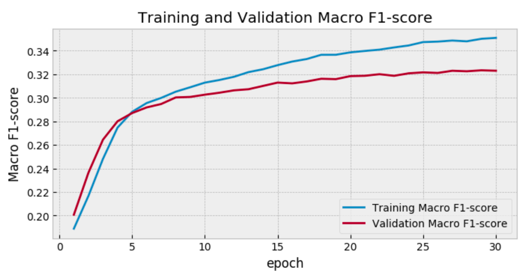
After 30 epochs, you may observe a convergence on the validation set.

Show predictions

Let’s see what the predictions look like when using our model on posters of some known movies in the validation set.

We notice that the model can get “Romance” right. Is it because of the red title on the poster of “An Affair of Love”?

What about the model suggesting new labels for “Clash of the Titans”? The “Sci-Fi” label seems very acurate and related to this film. Remember that in the original dataset a maximum of 3 labels are given for each poster. Probably, more useful labels could be recommended by using our model!

Export Keras model

After having trained and evaluated the model, you can export it as a TensorFlow saved model for future use.

from datetime import datetime
t = datetime.now().strftime("%Y%m%d_%H%M%S")
export_path = "./models/soft-f1_{}".format(t)
tf.keras.experimental.export_saved_model(model, export_path)
print("Model with macro soft-f1 was exported in this path: '{}'".format(export_path))

You can later reload the tf.keras model by specifying the path to the export directory containing the .pb file.

reloaded = tf.keras.experimental.load_from_saved_model(export_path,
                                                       custom_objects={'KerasLayer':hub.KerasLayer})

Notice the ‘KerasLayer’ object in the custom_objects dictionary. This is the TF.Hub module that was used in composing the model.

Summary

• Multi-label classification: When the number of possible labels for an observation is greater than one, you should rely on multiple logistic regressions to solve many independant binary classification problems. The advantage of using neural networks is that you can solve these many problems at the same time inside the same model. Mini-batch learning helps reduce memory complexity while training.
• TensorFlow data API: tf.data makes it possible to build fast input pipelines for training and evaluating TensorFlow models. Using the tf.data.Dataset abstraction, you can collect observations as a pair of tensor components representing the image and its labels, preprocess them in parallel and do the necessary shuffling and batching in a very easy and optimized manner.
• TensorFlow Hub: Transfer learning has never been this simple.
  TF.Hub provides reusable components from large pre-trained ML models. You could load a MobileNet feature extractor wrapped as a keras layer and attach your own fully connected layers on top of it. The pre-trained model can be frozen and only the weights of your classification layers get updated during training.
• Optimizing directly for macro F1: By introducing the macro soft-F1 loss, you could train the model to directly increase the metric you care about: the macro F1-score @ threshold 0.5.

The complete code can be found on GitHub. So, you can take a seat and get your hands on!

Originally published by Mohamed-Achref Maiza at https://towardsdatascience.com

#TensorFlow #MachineLearning #Ai