This tutorial is a concise step-by-step guide for building and training an Image Recognizer on any image dataset of your choice.
In this tutorial, you will learn how to:
- Scrape images from Google Images and create your own dataset
- Build and train an image recognizer on your dataset
- Visualize and adequately interpret classification results
- Test model with new images
To run this notebook, you can simply open it with Google Colab here.
Once in Colab, make sure to change the following to enable GPU backend,
Runtime -> Change runtime type -> Hardware Accelerator -> GPU
1. Image Dataset Download and Setup
Option 1: Working with a ready dataset of your own
If you would like to use your own image dataset for this tutorial, rearrange it in a way that images of the same class are under the same folder. Then, name the folders with the corresponding class labels.
Option 2: Scraping images from Google Images
If you do not have a dataset in-hand, you can scrape images from Google Images and make up a dataset of your choice. In order to do so, simply install Fatkun Batch Download Image extension on your google chrome browser and download any set of google images by clicking the extension tab. Place all images of the same class under the same folder and name it accordingly with the class label.
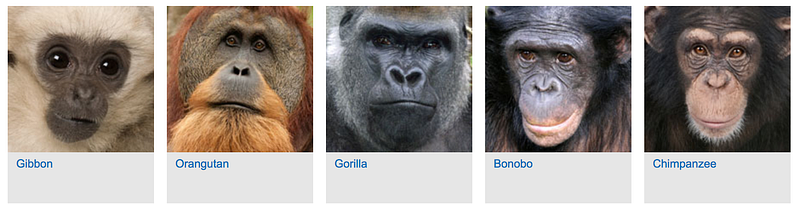
Option 3: Working with my Monkeys dataset, which I originally scraped from Google Images :)
The dataset can be downloaded and untarred using the following couple bash commands.
%%capture
	!wget "https://www.dropbox.com/s/35ithckx6vqryob/Monkeys_Faces_Dataset.tar?dl=0" -O Monkeys_Faces_Dataset.tar
	!tar --warning=no-unknown-keyword -xzf Monkeys_Faces_Dataset.tar
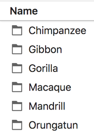
In this tutorial, we will be classifying Monkeys, so we created 6 folders corresponding to 6 different types of monkeys, as shown below.
If you choose to run this notebook with your dataset, simply replace the url and file name in the above cell with yours. Storing the .tar file in Dropbox worked best for me.
2. Image Recognition
For a further explanation of the code and functions used within this notebook, check out my other post: Concise Notes on Image Recognition, Fastai 2019 v3 Lesson 1
Initialization
%reload_ext autoreload %autoreload 2 %matplotlib inlinefrom fastai.vision import * from fastai.metrics import error_rate bs = 64 #batch size: if your GPU is running out of memory, set a smaller batch size, i.e 16 sz = 224 #image size PATH = './Monkeys Faces/'
PATH is the path containing all the class folders. You may keep ‘./Monkeys Faces’ if you are using Monkeys dataset. Otherwise, specify the path of your folders.
Let’s retrieve the image classes,
classes = []

for d in os.listdir(PATH):

if os.path.isdir(os.path.join(PATH, d)) and not d.startswith(‘.’):

classes.append(d)

print ("There are ", len(classes), “classes:\n”, classes)
There are  6 classes:

[‘Macaque’, ‘Orungatun’, ‘Chimpanzee’, ‘Gorilla’, ‘Mandrill’, ‘Gibbon’]
Let’s verify there are not any corrupt images that cannot be read. If found any, they will simply be deleted.
for c in classes:

print (“Class:”, c)

verify_images(os.path.join(PATH, c), delete=True);
Creating and training the classifier
Let’s create training and validation sets,
data  = ImageDataBunch.from_folder(PATH, ds_tfms=get_transforms(), size=sz, bs=bs, valid_pct=0.2).normalize(imagenet_stats)

print (“There are”, len(data.train_ds), “training images and”, len(data.valid_ds), “validation images.” )
There are 268 training images and 67 validation images.
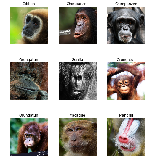
Let’s visualize some images from different classes,
data.show_batch(rows=3, figsize=(7,8))
Let’s build our Deep Convolutional Neural Network (CNN),
learn = cnn_learner(data, models.resnet34, metrics=accuracy)
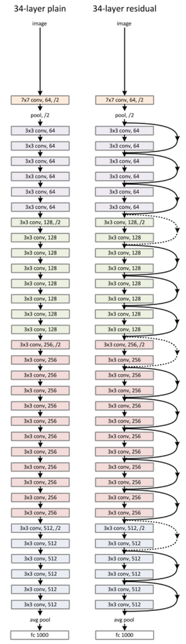
The CNN architecture used here is ResNet34. ResNet architecture has had great success within the last few years and still considered state-of-the-art, so I believe there is great value in discussing it a bit. If you are interested solely in getting the Image Recognizer to work, feel free to skip the next few paragraphs.
What is special about ResNet architecture is how it tackles the degradation problem most common in deep networks, where the model accuracy gets saturated and then degrades rapidly. It is important to note here that although some may assume that the core idea behind ResNets is overcoming the notorious vanishing gradient problem, where gradients get infinitely small as they back-propagate to earlier layers of the network, this is not quite true.
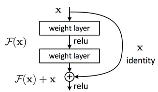
Resnet architecture introduces an “identity shortcut connection” or often referred to as a “skip connection”, which skips one or more layers. The shortcut connections simply perform identity mappings, and their outputs are added to the outputs of the stacked layers, as shown in the figure below. The skip function creates what is known as a residual block, F(x) in our figure, and that’s where the name Residual Nets (ResNets) came from.
Comprehensive empirical evidence has shown that the addition of these identity mappings allows the model to go deeper without degradation in performance and such networks are easier to optimize than plain stacked layers. There are several variants of ResNets, such as ResNet50, ResNet101, ResNet152; the number represents the number of layers (depth) of the ResNet.
In this tutorial, we are using ResNet34. Feel free to try any of the other ResNet models by simply replacing models.resnet34 above by models.resnet50 for instance, but bare in mind that increasing the number of layers would require more GPU memory.
Let’s now pick the appropriate learning rate parameter,
learn.lr_find();

learn.recorder.plot()
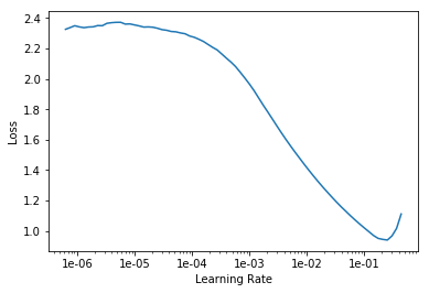
Use the above plot to pick adequate learning rates for your model. We need two learning rates since we are using cyclic learning rates:
- The first learning rate is just before the loss starts to increase, preferably 10x smaller than the rate at which the loss starts to increase. For instance, 1e-02 for our Monkeys dataset.
- The second learning rate is 10x smaller than the first learning rate, so 1e-03 in our example.
The plot will be different for your dataset, so make sure to pick these two learning rates accordingly.
Replace your chosen learning rates in the slice function below and let’s train the model.
learn.fit_one_cycle(4, max_lr=slice(1e-3,1e-2))
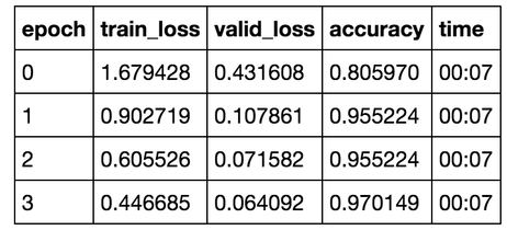
Great, we achieved a high classification accuracy with only a few lines of code and without much tuning of the parameters.
We are DONE but let’s further interpret the results.
3. Results Interpretation and Visualization
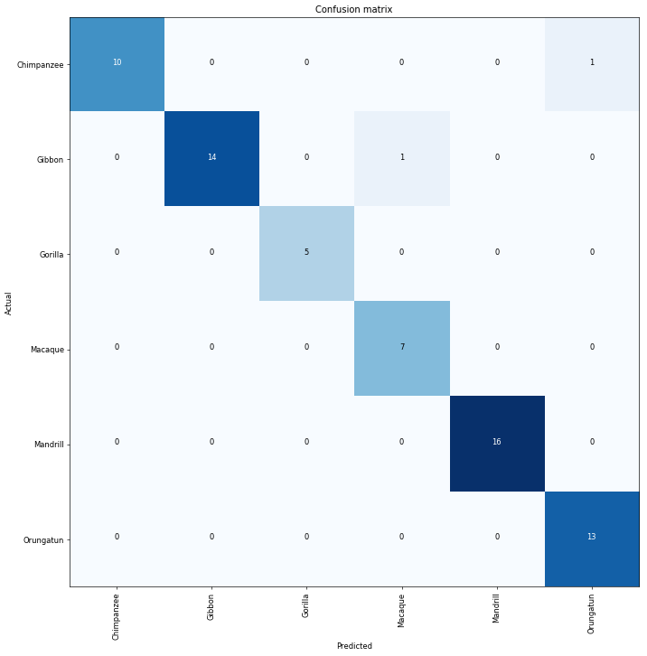
interp = ClassificationInterpretation.from_learner(learn)
We can start by visualizing a confusion matrix. The diagonal elements represent the number of images for which the predicted label is equal to the true label, while off-diagonal elements are those that are mislabeled by the classifier.
interp.plot_confusion_matrix(figsize=(12,12), dpi=60)
We can also plot images with top losses; in other words, the images that the model was most confused about. A high loss implies high confidence about the wrong answer.
interp.plot_top_losses(9, figsize=(15,11), heatmap=False)
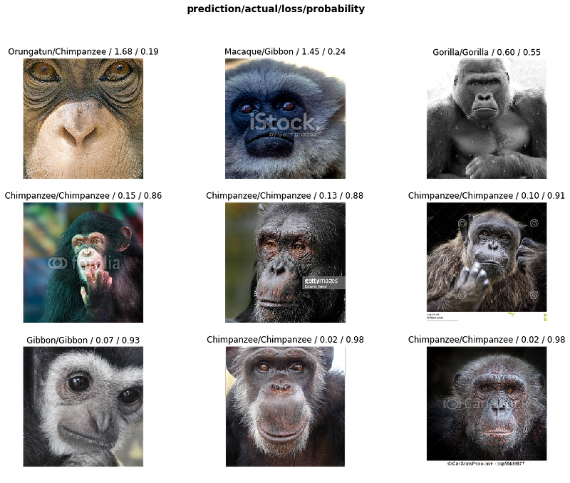
Images are shown along with top losses:
prediction label / actual label / loss / probability of actual image class.
4. Testing the model on a new image
Let’s now feed the model a new image it never seen before and see how well it classifies it.
Upload the image to the same folder of this notebook.
path = ‘./’ #The path of your test image

img = open_image(get_image_files(path)[0])

pred_class,pred_idx,outputs = learn.predict(img)

img.show()

print (“It is a”, pred_class)
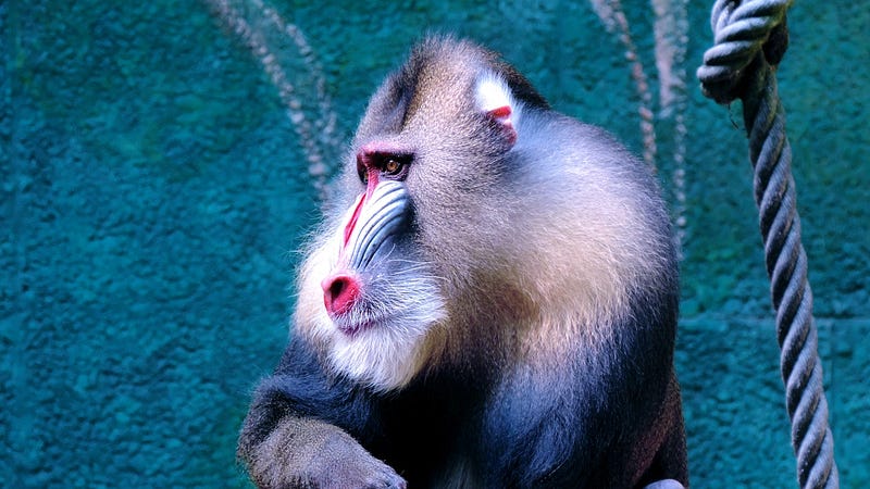
It is a Mandrill
Congratulations completing, reading, or skimming through this tutorial…
Originally published on https://towardsdatascience.com
#machine-learning #deep-learning #data-science #artificial-intelligence
