This blog is based on the notebook I used to submit predictions for Kaggle In-Class Housing Prices Competition. My submission ranked 293 on the score board, although the focus of this blog is not how to get a high score but to help beginners develop intuition for Machine Learning regression techniques and feature engineering. I am a final year mechanical engineering student, I started learning python in January 2020 with no intentions to learn data science. Thus, any suggestions in the comments for improvement will be appreciated.

The data set contains houses in Ames, Iowa. Photo by chuttersnap on Unsplash

Introduction

The scope of this blog is on the data pre-processing, feature engineering, multivariate analysis using Lasso Regression and predicting sale prices using cross validated Ridge Regression.

The original notebook also contains code on predicting prices using a blended model of Ridge, Support Vector Regression and XG-Boost Regression, which would make this blog verbose. To keep this blog succinct, code blocks are pasted as images where necessary.

The notebook is uploaded on the competition dashboard if reference or code is required : https://www.kaggle.com/devarshraval/top-2-feature-selection-ridge-regression

This data set is of particular importance to novices like me in the sense of the vast range of features. There are a total of 79 features(excluding Id) which are said to explain the sale price of the house, it tests the industriousness of the learner in handling these many features.

1. Exploratory data analysis

The first step in any data science project should be getting to know the data variables and target. This stage can make one quite pensive or other hand feel enervated depending on one’s interests. Exploring the data gives an understanding of the problem and feature engineering ideas.

It is recommended to read the feature description text file to understand feature names and categorize the variables into groups such as Space-related features, Basement features, Amenities, Year built and remod, Garage features, and etc based on subjective views.

This categorization and feature importance becomes more intuitive after a few commands in the notebook such as:

corrmat=df_train.corr()
corrmat['SalePrice'].sort_values(ascending=False).head(10)

SalePrice 1.000000

OverallQual 0.790982

GrLivArea 0.708624

GarageCars 0.640409

GarageArea 0.623431

TotalBsmtSF 0.613581

1stFlrSF 0.605852

FullBath 0.560664

TotRmsAbvGrd 0.533723

YearBuilt 0.522897

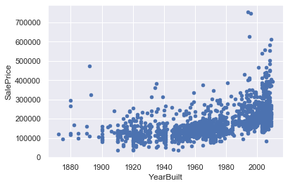
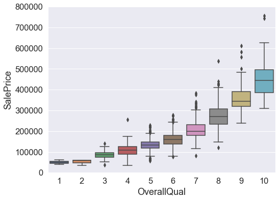
Naturally, overall quality of the house is strongly correlated with the price. However, it is not defined how this measure was calculated. Other features closely related are space considerations (Gr Liv Area, Total Basement area, Garage area) and how old the house is (Year Built).

The correlations give an univariate idea of important features. Thus, we can plot all of these features and remove outliers or multicollinearity. Outliers can skew regression models sharply and multicollinearity can undermine importance of a feature for our model.

1.1 Multi-collinearity

f, ax = plt.subplots(figsize=(10,12))
sns.heatmap(corrmat,mask=corrmat<0.75,linewidth=0.5,cmap="Blues", square=True)

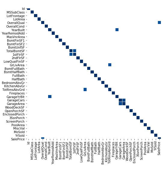
The Seaborn heatmap shows features with correlation above 75%

Thus, highly inter-correlated variables are:

1. GarageYrBlt and YearBuilt
2. TotRmsAbvGrd and GrLivArea
3. 1stFlrSF and TotalBsmtSF
4. GarageArea and GarageCars

GarageYrBlt, TotRmsAbvGrd, GarageCars can be deleted as they give the same information as other features.

1.2. Outliers

First, examine the plots of features versus target one by one and identify observations that do not follow the trend. Only these observations are outliers and not the ones following the trend but having a greater or smaller value.

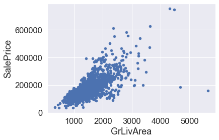
#Outliers in Fig 1 
df_train.sort_values(by = 'GrLivArea', ascending = False)[:2]
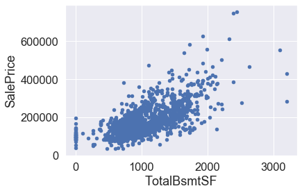
#Fig 2(Clockwise)
df_train.sort_values(by='TotalBsmtSF',ascending=False)[:2]
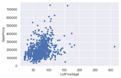
#fig 3 
df_train.drop(df_train[df_train['LotFrontage']>200].index,inplace=True)
#Fig 4
df_train.drop(df_train[(df_train.YearBuilt < 1900) & (df_train.SalePrice > 200000)].index,inplace=True)
## Fig 5
df_train.drop(df_train[(df_train.OverallQual==4) & (df_train.SalePrice>200000)].index

One might be tempted to delete the observations for LotArea above 100k. However, on second thought it is possible these were just large houses but overall low quality.

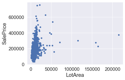
df_train[df_train['LotArea']>100000]['OverallQual']

Out []:
249    6
313    7
335    5
706    7

Thus, we see that despite having larger Lot Area, these houses have a overall quality of 7, and average price for that quality is a bit more than 200k as seen in the box plot. Thus, these houses may not be a harmful outlier to the model.

Thus, we will see the correlations will have increased for the variables after removing outliers.

#feature-engineering #kaggle-competition #regression #data-science #feature-selection