I like tower defense games and was thinking about trying my hand at making one. But while I was making a mental checklist of things I’d need for it, it occurred to me that I would need to study pathfinding algorithms. I didn’t know the best place to start, so I went with a Google search and found the A* algorithm. Neat algorithm, but I did find plenty of notes saying that it was sort of a descendant of Dijkstra’s algorithm, and I found that was a better starting point.
You might want to know a bit about data structures, nodes, and graphs before going into this, but even if you do not, I’ll do my best to bring in as many visuals as I can and keep each step as clear as possible. I’ll also list all the references I found, and credit them as much as I can, because I am totally going to be stealing their examples.
Set-up
I’ve looked at lot of of graphs today, but I think this is the best and simplest for demonstrating Dijkstra’s algorithm. Just five nodes, or vertices because this is a graph, each with two to four edges.
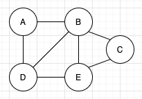
“Karl, you even labeled the vertices the same as your source! That’s plagiarism!” Nonsense, I labeled them A through E, left to right, top to bottom. And so did they! Great minds think a like!
Right now, I could ask you what the quickest way from A to C would be is, and you might see that the best path is A to B to C. But graphs are commonly abstractions of some relationship, and in the case of pathfinding, the vertices are specific locations and the edges are the distances between them. So what if we represented longer distances between vertices with longer edges, something like this:
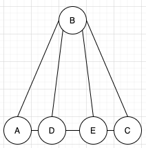
As far as graph theory and topology are concerned, this graph is identical to the first one. All the vertices still point to the same vertices as before, but some of the edges are longer and some are shorter. Also, the shortest distance between A and C now passes through D and E.
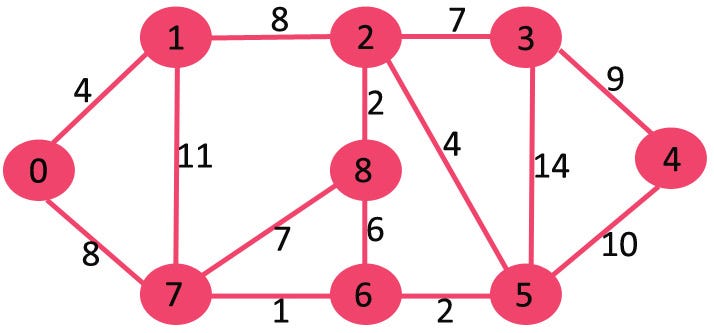
However, having a graph that is more visually accurate of what it’s representing is not particularly useful in computing anything. Unsurprisingly, the best way to make this graph more algorithmically friendly is to add numbers to it, in the form of weights for the edges.
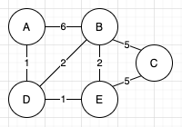
The numbers on the edges are called weights, and they’ll represent some value about the relationship between the two vertices. In pathfinding, this will likely be distance. Again, because of the smaller weights, the shortest distance between A and C is still A > D > E > C.
This will be the graph, vertices, and weights I’ll be using for the rest of this article. The goal will be using Dijkstra’s algorithm to find the shortest path between vertices A and C. To do this, I’ll need just a few extra things; some for helping the algorithm, and some to act as visual aides. On the algorithm side, I need two sets to hold the vertices, one called “visited” and one called “unvisited”. The algorithm is going to work through the unvisited vertex set, one at a time, and when it’s done with each vertex, it will place them in the visited set. On the visual aide side, I’ll want a table of all the vertices, to keep track of their shortest distance from vertex A, and the first vertex that was in-between them and vertex A. The final set-up will look something like this:
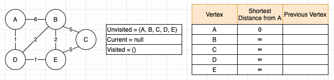
A few more things to note here: I’ve jumped ahead a bit and filled in the initial shortest distances. Vertex A starts at zero because if your starting point and ending point are the same, there is no distance to travel. For the rest of the vertices, the distances are initially unknown, and until those are visited and evaluated, they’ll start off as infinity. Second thing to note is that I added a “current” field. This is a more of a visual aide thing to let you know which vertex is currently being visited. And third, this set-up is wholesale theft. I have no excuse for this one, but I’ll leave a link to my source in the references.
Stepping Through the Algorithm
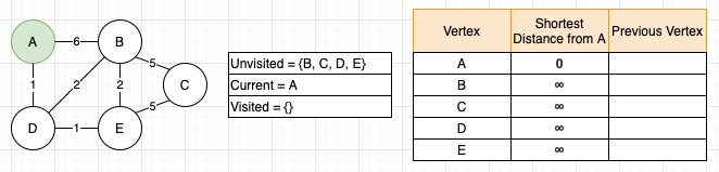
The first step of the algorithm is to go through the unvisited vertices and look for the one with the shortest distance from A. At the start, everything is unvisited, and the only vertex with a known distance is A, so we start by examining A.
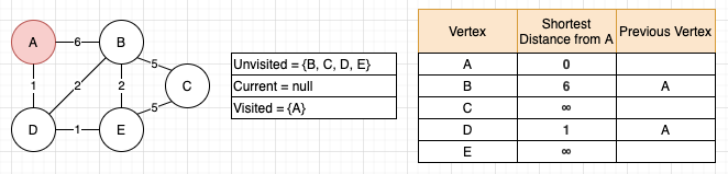
Now that we have a current vertex, we need to look at its unvisited neighbors, which in this case are vertices B and D. For each unvisited neighbor, we need to find their distance from vertex A. This will be more complicated later, but because we are currently measuring directly from A to these vertices, it will just be the weights on those edges: A to B is 6, and A to D is 1. With these two values in hand, we need to compare them to the current recorded shortest distance from vertex A, and if the new distance is smaller, replace that value. On the table, we can see that both B and D are still set to infinity, so 6 and 1 are definitely smaller and will be made the new shortest distance. Alongside updating the distance, we also need to record that this new shortest distance was made by a connection through the current vertex. Again, this feels silly on the first loop when it’s a clear, direct connection to A, but this is what makes the algorithm work. Finally, we can move A to the visited set, and that is one loop of the algorithm.
Rinse and Repeat
And now we start all over, going through the same steps and following the same rules. So, look at the unvisited set and find the one with the shortest distance from A. More choices this time around, but D, with a distance of 1, is clearly the shortest, so it will be the new current vertex.
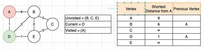
Just like before, we now need to look at D’s unvisited neighbors, which are B and E. A is also a neighbor, but because it has been visited already and is in the visited set, it will not be examined, affected, or changed here. Next, we need the distance from the neighbors to A. Using E as an example, the distance from D to E on the graph is 1, and D’s shortest distance from A on the table is 1, so 1+1=2. Before, in the first loop with B and D, this would’ve looked like 0+6 and 0+1, because A was the current vertex and its shortest distance was 0. However, writing out 0+1 in that first pass just looks odd to me, so I passed over explaining it like this until now as I think it makes a little more sense on every iteration after the first.
#dijkstra #pathfinding #algorithms #graph #algorithms