Build Your Own Image Classifier In Tensorflow

Convolutional Neural Network (CNN) is a special type of deep neural network that performs impressively in computer vision problems such as image classification, object detection, etc. In this article, we are going to create an image classifier with Tensorflow by implementing a CNN to classify cats & dogs.

With traditional programming is it not possible to build scalable solutions for problems like computer vision since it is not feasible to write an algorithm that is generalized enough to identify the nature of images. With machine learning, we can build an approximation that is sufficient enough for use-cases by training a model for given examples and predict for unseen data.

How CNN work?

CNN is constructed with multiple convolution layers, pooling layers, and dense layers.

The idea of the convolution layer is to transform the input image in order to extract features (ex. ears, nose, legs of cats & dogs) to distinguish them correctly. This is done by convolving the image with a kernel. A kernel is specialized to extract certain features. It is possible to apply multiple kernels to a single image to capture multiple features.

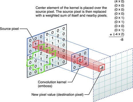
How kernel is applied to an image to extract features

Usually, an activation function (ex. tanh, relu) will be applied to the convoluted values to increase the non-linearity.

The job of the pooling layer is to reduce the image size. It will only keep the most important features and remove the other area from the image. Moreover, this will reduce the computational cost as well. The most popular pooling strategies are max-pooling and average-pooling.

The size of the pooling matrix will determize the image reduction. Ex. 2x2 will reduce the image size by 50%

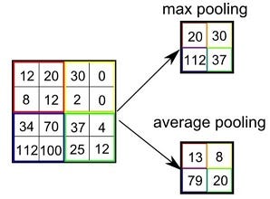
How max-pooling and average-pooling works

These series of convolution layers and pooling layers will help to identify the features and they will be followed by the dense layers for learning and prediction later.

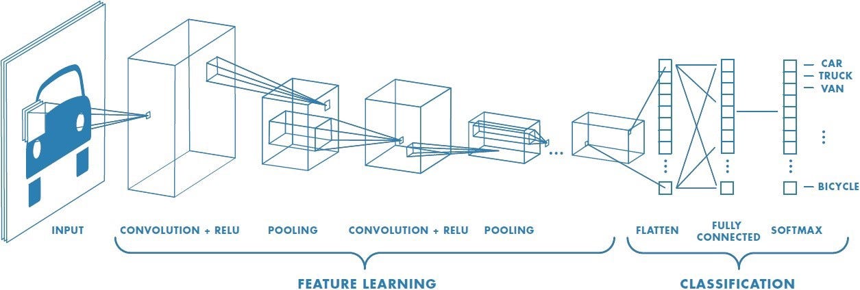
Layers of a CNN

Building the Image Classifier

CNN is a deep neural network that needs much computation power for training. Moreover, to obtain sufficient accuracy there should be a large dataset to construct a generalized model for unseen data. Hence here I am running the code in Google Colab which is a platform for research purposes. Colab supports GPU enabled hardware which gives a huge boost for training as well.

Download and load the dataset

This dataset contains 2000 jpg images of cats and dogs. First, we need to download the dataset and extract it (Here data is downloaded to /tmp directory in Colab instance).

Downloading dataset

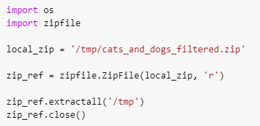
Extracting the dataset

The above code segments will download the datasets and extract them to /tmp directory. The extracted directory will have 2 subdirectories named train and validation. Those will have the training and testing data. Inside both those directories, there are 2 subdirectories for cats and dogs as well. We can easily load these training and testing data for the 2 classes with the TensorFlow data generator.

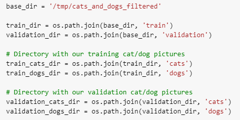
Setting the paths of testing and validation images

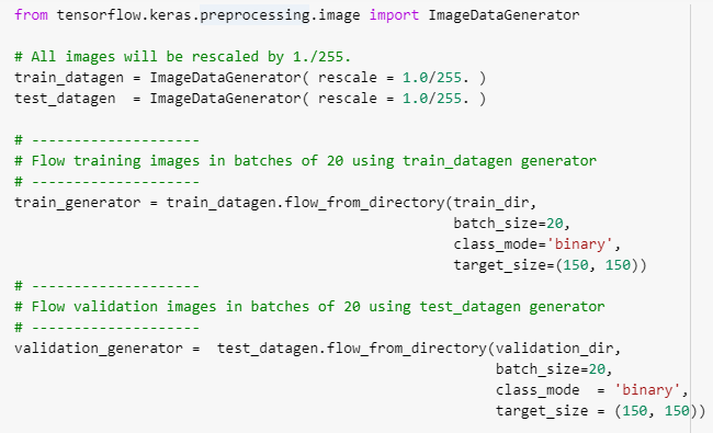
Load data with Ternsorflow image generator

Here we have 2 data generators for train and test data. When loading the data a rescaling is applied to normalize the pixel values for faster converging the model. Moreover, when loading the data we do it in 20 image batches and all of them are resized into 150x150 size. If there are images in different sizes this will fix it.

Constructing the model

Since the data is ready, now we can build up the model. Here I am going to add 3 convolutional layers followed by 3 max-pooling layers. Then there is a Flatten layer and finally, there are 2 dense layers.

Construct the CNN model

In the first convolution layer, I have added 16 kernels which have the size of 3x3. Once the image is convoluted with kernel it will be passed through relu activation to obtain non-linearity. The input shape of this layer should be 150x150 since we resized images for that size. Since all the images are colored images, they have 3 channels for RGB.

In the max-pooling layer, I have added a 2x2 kernel such that the max value will be taken when reducing the image size by 50%.

There are 3 such layers (convolution and max-pooling) to extract the features of images. If there are very complex features that need to be learned, more layers should be added to the model making it much deeper.

The Flatten layer will take the output from the previous max-pooling layer and convert it to a 1D array such that it can be feed into the Dense layers. A dense layer is a regular layer of neurons in a neural network. This is where the actual learning process happens by adjusting the weights. Here we have 2 such dense layers and since this is a binary classification there is only 1 neuron in the output layer. The number of neurons in the other layer can be adjusted as a hyperparameter to obtain the best accuracy.

Train the model

Since we have constructed the model, now we can compile it.

Compile the model

Here we need to define how to calculate the loss or error. Since we are using a binary classification we can use binary_crossentropy. With the optimizer parameter, we pass how to adjust the weights in the network such that the loss gets reduced. There are many options that can be used and here I use the RMSprop method. Finally, the metrics parameter will be used to estimate how good our model is and here we use the accuracy.

Now we can start training the model

Train the model

Here we are passing the train and validation generators we used to load our data. Since our data generator has 20 batch size we need to have 100 stps_per_epoch to cover all 2000 training images and 50 for validation images. The epochs parameter sets the number of iterations we conduct for training. The verbose parameter will show the progress in each iteration while training.

Results

Results after 15 epochs

After 15 epochs the model has scored 98.9% accuracy on training set and 71.5% accuracy on the validation set. This is a clear indication that our model has overfitted. Our model will perform really good in the training set and it will poorly perform for the unseen data.

To solve the overfitting problem either we can add regularization to avoid over-complexing the model or we can add more data to the training set to make the model more generalized for unseen data. Since we have a very small data set (2000 images) for training, adding more data should fix the issue.

Collecting more data to train a model is overwhelming in machine learning since it is required to preprocess the data again. But when working with images, especially in image classification, there is no need to collect more data. This can be fixed the technique called Image Augmentation.

Image Augmentation

The idea of Image Augmentation is to create more images by resizing, zooming, rotating images, etc to construct new images. With this approach, the model will able to capture more features than before and will able to generalize well for unseen data.

For example, let’s assume most of the cats in our training set as follows which have the full body of a cat. The model will try to learn the shape of the body of the cat from these images.

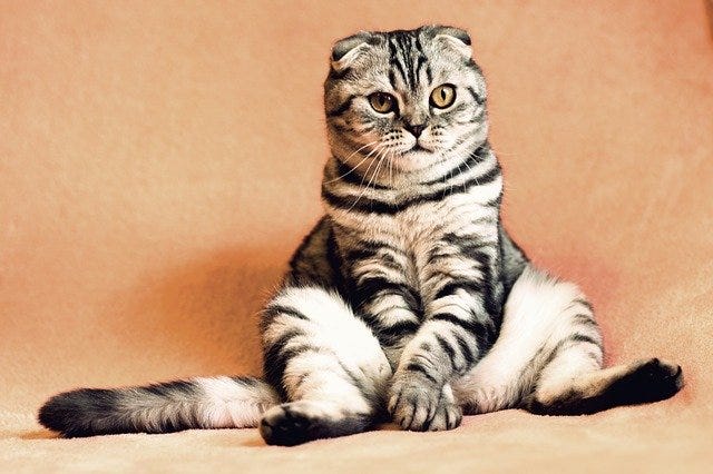
Due to this, the classifier might fail to identify images like follow correctly since it hasn’t trained with examples similar to that.

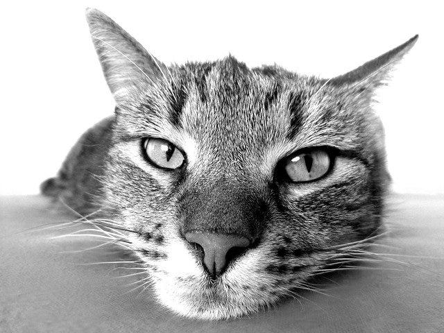
But with image augmentation, we can construct new images from existing images to make the classifier learn new features. With the zoom feature in image augmentation, we can construct a new image like below to help the learner to classify images like above which failed to classify correctly before

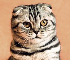
Zoomed image from the original image with image augmentation

Adding image augmentation is really easy with the TensorFlow image generator. When image augmentation is applying, the original dataset will be untouched and all the manipulations will be done in the memory. The following code segment will show how to add this functionality.

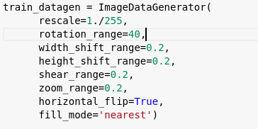
Adding image augmentation when loading data

In here image rotating, shifting, zooming and few other image manipulation techniques are applied to generate new samples in the training set.

Once we apply the image augmentation it is possible to obtain 86% training accuracy and 81% testing accuracy. As you can see this model is not overfitted like before and with a very small dataset like this, this accuracy is impressive. Further, you can improve the accuracy by playing with the hyperparameters like the optimizer, the number of dense layers, number of neurons in each layer, etc.

#tensorflow #ai