Table of Contents:

1. Business Problem
2. Problem Statement
3. Data Preparation
4. Exploratory Data Analysis
5. Feature Engineering
6. Data Preprocessing
7. Feature Selection
8. Modeling
9. Summary
10. Predictions on Test Data
11. Conclusion and Future Work
12. References

1. Business Problem:

Vehicle Testing is an important aspect in the automobile manufacturing process. Every vehicle must pass a certain standard before it is delivered to the customer. Mercedes Benz offers a wide range of vehicles with different customization. Each vehicle must undergo testing in order to ensure vehicle satisfies the safety requirements and meets the emission norms. Each model requires a different test stand configuration due to the customization. Since the number of models are more, large number of tests need to be conducted. More tests result in more time spent on the test stand increasing costs for Mercedes-Benz and generating higher carbon dioxide (green house pollutant gas).

The Mercedes Benz Green Manufacturing Competition hosted on Kaggle intends to optimize the vehicle testing process by developing a machine learning model which can predict the time spent by a vehicle on test stand. The ultimate goal is to reduce the time spent on a test stand which will result in reduced carbon dioxide emissions during testing phase. The dataset for this study is provided by Mercedes Benz. The data can be downloaded from this link.

2. Problem Statement:

The task is to develop a machine learning model that can predict the time a car will spend on the test bench based on the vehicle configuration. The vehicle configuration is defined as the set of customization options and features selected for the particular vehicle. The motivation behind the problem is that an accurate model will be able to reduce the total time spent on testing vehicles by allowing cars with similar testing configurations to be run successively. This problem is a supervised machine learning regression task since it involves predicting a continuous target variable based on a bunch of independent variables by learning for a labelled training data.

The evaluation metric is R-squared also known as co-efficient of determination. It quantifies the percentage of variation in target variables that is explained by the features. R-squared value can lie between 0 and 1. The best possible value of R-squared is 1 which indicates that all the variation in target variables is explained by the input features.

3. Data Preparation:

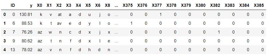
Two datasets are provided by Mercedes-Benz for this competition namely train.csv and test.csv. The file train.csv is the labeled dataset on which machine learning model has to be developed. The file test.csv is the dataset on which predictions are to be made. Both training and test data contain 377 features which represent the vehicle configuration during the vehicle testing phase. The features have names such as ‘X0’, ‘X1’, ‘X2’ and so on. There is a feature ‘ID’ which represents the ID assigned to each vehicle test. The features are anonymous and do not have any physical representation. The description of the data states that these features are configuration options such as suspension setting, adaptive cruise control, all-wheel drive and a number of different options that together define a car model. A subset of training data in shown in image below.

#Load dataset
data = pd.read_csv('train.csv')
data.head()

There are 377 features out of which 368 are binary, 8 are categorical and 1 is continuous. The target variable y is continuous value which represents the time taken by vehicle for testing in seconds. There are no missing values present in the dataset. The train.csv file is split into training and validation set. Below image shows the code for this operation.

#Separate the dependent and independent features
X = data.drop(columns=['y'])
Y = data['y']

#Split the dataset
X_train, X_val, y_train, y_val = train_test_split(X, Y, 
test_size=0.2, random_state=25)
#Concatenate X_train and y_train
train_data = pd.merge(X_train,y_train.to_frame(),left_index=True, right_index=True)
train_data.head()

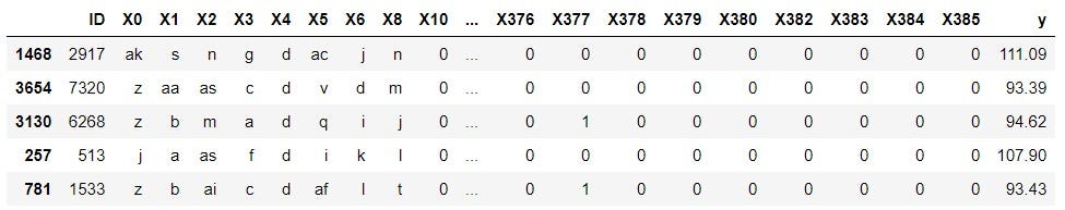
Exploratory Data Analysis (EDA) is performed on train_data mentioned in above code.

4. Exploratory Data Analysis:

4.1. Analyze target/dependent variable:

Below image contains the histogram and box-plot of target variable.

The target variable has a mean of 100 seconds. Points with target values above 137.5 can be inferred as outlier points from boxplot. For this competition, points above 150 are classified as outlier points and they are removed from the training set.

4.2. Analyze categorical variables:

There are 8 categorical features namely X0, X1, X2, X3, X4, X5, X6, and X8. For each of these features histogram of counts of unique values and boxplot of unique values is plotted.

4.2.1. X0 feature:

Observations from above plots:

1. aa, ab, g and ac occur only once.
2. The box-plots of z, y, t, o, f, n, s, al, m, ai, e, ba, aq, am, u, i, ad and b are nearly same. The mean of these categories is nearly 93.
3. The box-plots of ak, x, j, w, af, at, a, ax, i, au, as, r and c are nearly same. The mean of these categories is nearly 110.
4. Thus there appears to be grouping among different categories of X0.

4.2.2. X1 feature:

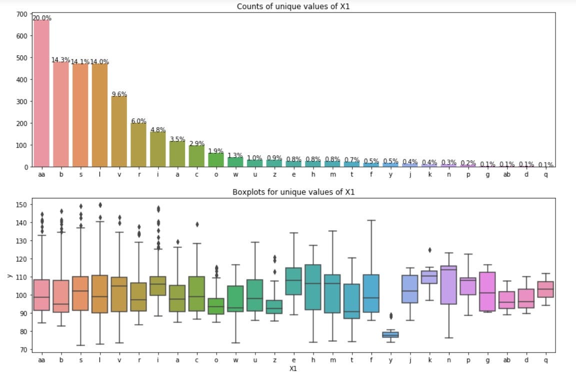
Observations from above plots:

1. Most of the categories of X1 have mean of 100.
2. y of X1 category is clearly separated from rest of the categories.

4.2.3. X2 feature:

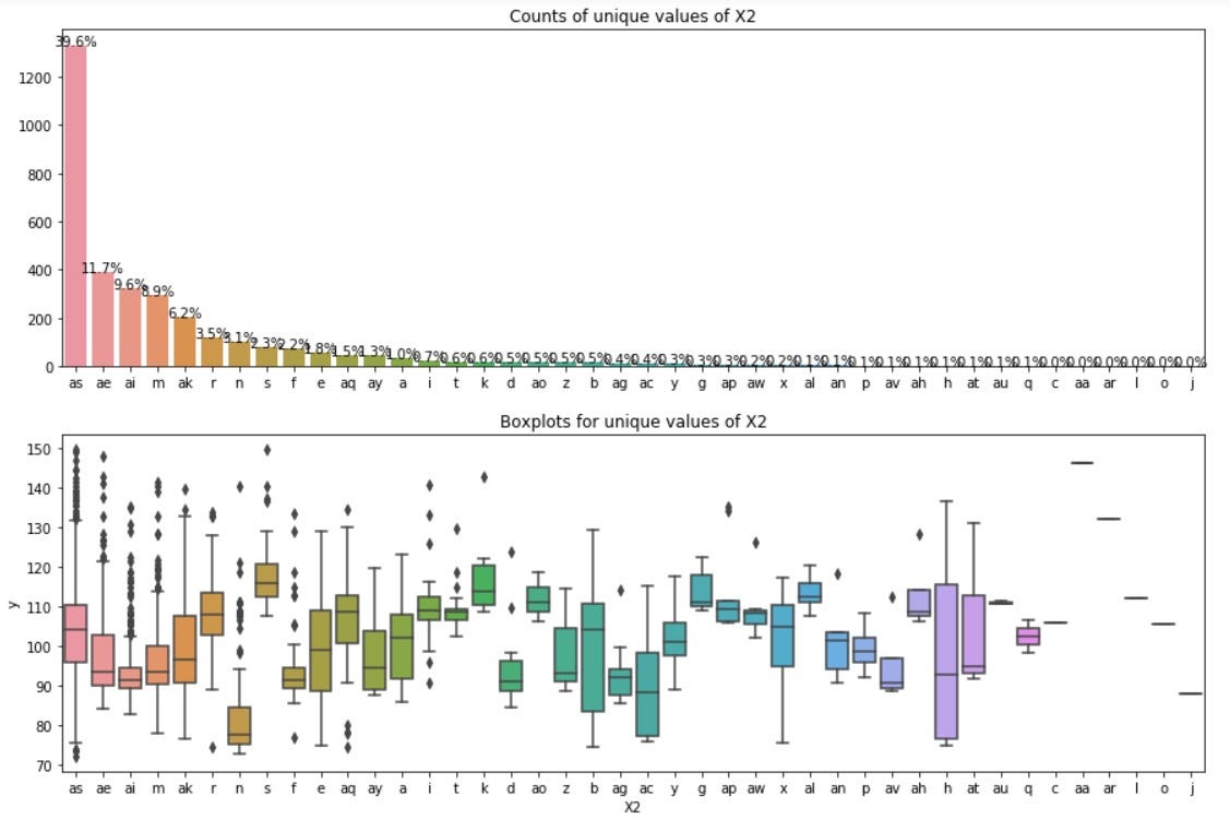
Observations from above plots:

1. ae category dominates in X2. 39% values of X2 are ae.
2. Similar to X0 there appears to be grouping in X2. X2 has less grouping than X0.
3. Most of categories of X2 have mean close to 97.

4.2.4. X3 feature:

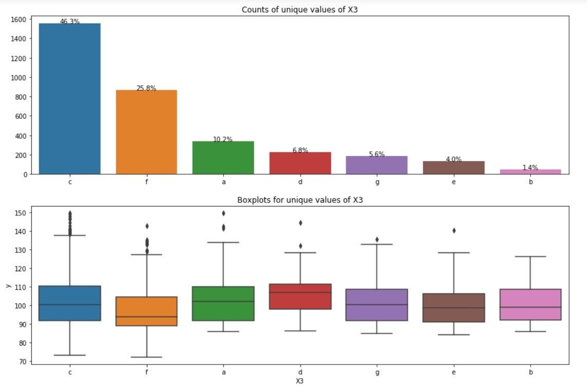
Observations from above plots:

1. c category dominates in X3. 46% values of X3 are c.
2. Almost all the categories of X3 have mean of 100.
3. There appears to be less variation in dependent variable y across the categories of X3. The box-plots for most of the categories of X3 match.

4.2.5. X4 feature:

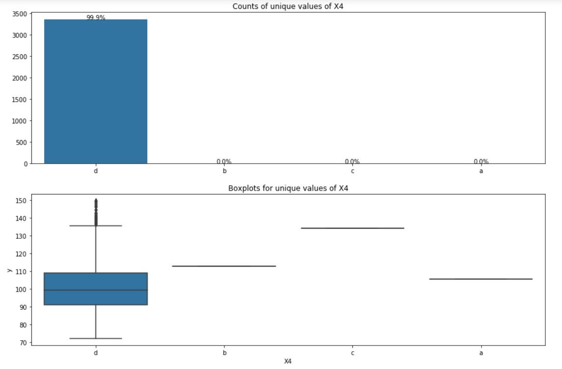
Observations from above plots:

1. d category dominates in X4. 99.9% values of X4 are d.
2. This feature must be dropped as there is no variance present in the feature.

4.2.6. X5 feature:

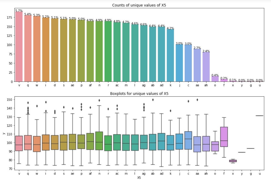
Observations from above plots:

1. x, h, g, y and u occur very rarely in the data.
2. The mean of all categories of X5 is close to 98.
3. There appears to be less variation in dependent variable y across the categories of X5. The boxplots for most of the categories of X5 match.

#deep-learning #machine-learning #kaggle #stacking #top-5 #deep learning