Machine learning using TensorFlow for Absolute Beginners

Welcome to this article where you will learn how to train your first Machine Learning model using TensorFlow and use it for Predictions! As the title suggests, this tutorial is only for someone who has no prior understanding of how to use a machine learning model.

The only pre-requisite for this course is to have a basic understanding of Python programming language. I have tried to keep things simple here, and only introduce basic concepts of machine learning and Neural Network.

What is TensorFlow: TensorFlow is an end-to-end open source platform for machine learning. It has a comprehensive, flexible ecosystem of tools, libraries and community resources that lets researchers push the state-of-the-art in ML and developers easily build and deploy ML powered applications. Learn more about TensorFlow from here.

We will be using Google Colab for this demo. Google Colab is a free cloud service which can be used to develop deep learning applications using popular libraries such as Keras, TensorFlow, PyTorch, and OpenCV. To know more about Google Colab, click here.

Let’s jump straight to a sample problem we are going to solve using TensorFlow and Machine-Learning concepts.

Let’s assume that we are given the marketing budget spent (in thousands of dollars) by a media-services provider in the last 8 months along with the number of new subscribers(also in thousands) for the same period of time in the table given below:

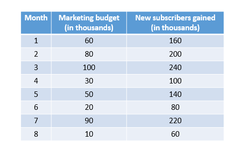
Table containing the data

As you can see there is a trend or relationship between the amount spent and new subscribers gained. As the amount is increasing, the number of new subscribers are also increasing.

If you work out the maths using theory of linear equation you will find out:

Subscribers gained = 2Amount Spent+ 40*
Our goal is to find this relationship between the amount spent on marketing and the number of subscribers gained using Machine-Learning technique.

Using the relationship found above we can also predict how many new subscribers can be expected if the organization spends some ‘x’ amount on marketing.

Let’s learn about some basic Machine Learning terminology before jumping into our modeling process:

Feature:* The input(s) to our model. In this case, a single value — marketing Budget.> Labels: The output our model predicts. In this case, a single value — the number of new subscribers gained.> Example: A pair of inputs/outputs used during training. In our case a pair of values from <em>mar_budget</em> and <em>New_subs</em> at a specific index, such as (80,200).*> ***Model: ***A mathematical representation of a real-world process. In machine Learning a model is an artifact or entity which is created by using a class of algorithm and training it with Features and labels.
Now let’s start with our Modeling Process.

Step 1: Creating a new Notebook

Click on the link below to visit colab and click on** File**, then** New python 3 notebook**.

https://colab.research.google.com/notebooks/welcome.ipynb

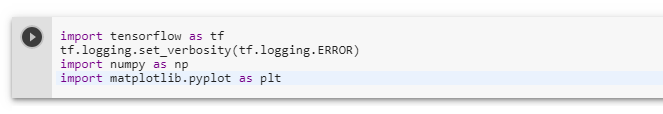
Step 2: The second step is to import Dependencies/libraries we are going to use in this Demo:

import numpy, matplotlib and tensorflow as given in the snippet below:

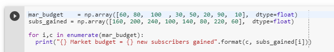
Step 3: Generate/Import the set of Data-Points

Let’s Generate a set of Data-Points we will be using to train our model in the form of two arrays named Mar_budget and Subs_gained for each value in mar_budget respectively.

We will also plot our arrays to understand the relationship between mar_budget and Subs_gained.

We’ll use [Matplotlib] to visualize this (you could use another tool).

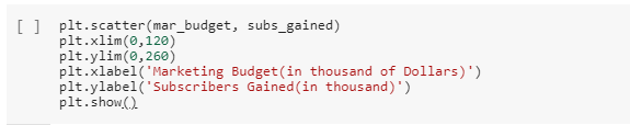
                code for plotting the Graph

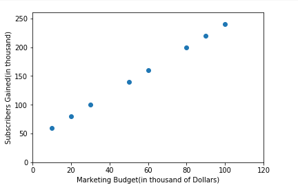
As you can see, there is a linear relationship between the Marketing Budget spent and new Subs Gained. Our Goal will be to find the equation of the line that can be used to fit all the points i.e explain this linear Relationship and later used to predict labels for unseen data points/predictors.

(Note: The relationship between data need not be always perfectly linear. In this example, I am using perfectly linear datapoints but in real life scenarios, there is hardly any dataset which is perfectly linear. Our goal is to find the most approximate line/Curve also called Model, that can be used to explain the relationship between predictors and labels. You can also generate or use Non-Linear Datapoints for this case study. )

I will take this opportunity to explain the principle assumption of linear regression which is:

Principle assumption of Linear Regression: There must be a linear Relationship between labels and Coefficients of the equation of line fitted.

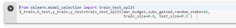
Step 4: The next step is to separate our data into training and testing Data. Training Data is used to train our model while testing data will be kept separately and later used for verifying the performance of our Model by comparing the actual Label of our test data with label predicted by our model for test data.

Step 5: Creating the model

We will use the simplest possible model we can, a Dense network. Since the problem is straightforward, this network will require only a single layer, with a single neuron.

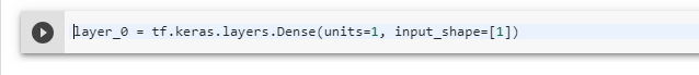
Build a layer:

We’ll call the layer layer_0 and create it by instantiating tf.keras.layers.Densewith the following configuration:

• input_shape=[1]: This specifies that the input to this layer is a single value. That is, the shape is a one-dimensional array with one member. Since this is the first (and only) layer, that input shape is the input shape of the entire model. The single value is a floating point number, representing marketing_budget.
• units=1: This specifies the number of neurons in the layer. The number of neurons defines how many internal variables the layer has to try to learn how to solve the problem. Since this is the final layer, it is also the size of the model’s output — a single float value representing new subscribers gained. (In a multi-layered network, the size and shape of the layer would need to match the input_shape of the next layer.)

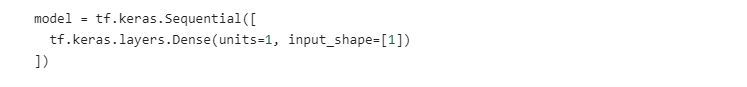
Assemble layers into the model:

Once layers are defined, they need to be assembled into a model. The Sequential model definition takes a list of layers as arguments specifying the calculation order from the input to the output.

This model has just a single layer, layer_0.

Note: You will often see the layers defined inside the model definition, rather than beforehand as below:

Step 6: Compile the model, with loss and optimizer functions

Before training, the model has to be compiled. When compiled for training, the model is given:

• Loss function: A way of measuring how far off predictions are from the desired outcome. (The measured difference is called the “loss”.)
• Optimizer function: A way of adjusting internal values in order to reduce the loss.

These parameters are used during training (model.fit(), below) to first calculate the loss at each point, and then improve it. In fact, the act of calculating the current loss of a model and then improving it is precisely what training is.

During training, the optimizer function is used to calculate adjustments to the model’s internal variables. The goal is to adjust the internal variables until the model (which is really a math function) mirrors the actual equation for converting budget_Spent to New Subs Gained.

TensorFlow uses numerical analysis to perform this tuning, and all this complexity is hidden from you so we will not go into the details here. What is useful to know about these parameters are:

The loss function (mean squared error) and the optimizer (Adam) used here are standard for simple models like this one, but many others are available. It is not important to know how these specific functions work at this point.

One part of the Optimizer you may need to think about when building your own models is the learning rate (0.1 in the code above). This is the step size taken when adjusting values in the model. If the value is too small, it will take too many iterations to train the model. Too large, and accuracy goes down. Finding a good value often involves some trial and error, but the range is usually within 0.001 (default), and 0.1.

To read more about loss Function and Optimizer click on the links given below:

• Mean squared error
• Adam

Step 7: Train the model by calling the fit method.

During training, the model takes in marketing budget values, performs a calculation using the current internal variables (called “weights”) and outputs values which are meant to be the New subs Gained. Since the weights are initially set randomly, the output will not be close to the correct value. The difference between the actual output and the desired output is calculated using the loss function, and the optimizer function directs how the weights should be adjusted.

This cycle of calculating, comparing, adjusting is controlled by the fit method. The first argument is the inputs, the second argument is the desired outputs.

The* *epochs argument specifies how many times this cycle should be run, and the verbose argument controls how much output the method produces.

Optional Step: Display training statistics

The fit method returns a history object. We can use this object to plot how the loss of our model goes down after each training epoch. A high loss means that the value of new subs gained the model predicts, are far from the corresponding value of*** actual subs gained***.

As you can see, our model improves very quickly at first and then has a steady, slow improvement until it is very near “perfect” towards the end:

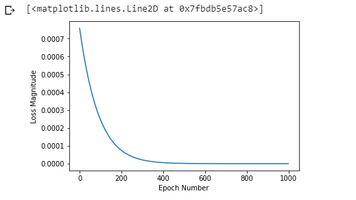
Epochs vs Loss

Step 8: Use the model to predict values

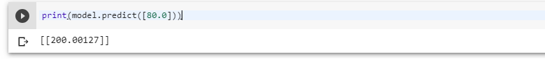
Now you have a model that has been trained to learn the relationship between marketing_Budget and new_subs_gained. You can use the predict method to have it calculate the new_subs_gained for a previously known/unknown marketing_budget.

So, for example, if the marketing_budget value is 80 thousand dollars, what do you think the new_subs_gained result will be?

Take a guess before you run this code or refer to your train_data:

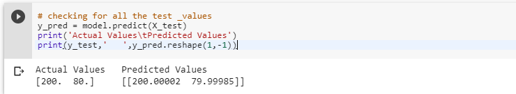
Next, we will predict labels for all test data points and compare them with their actual data points:

Step 9: Verifying the Model accuracy using Performance Metric

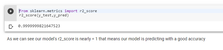
Let’s check the goodness of fit for model using r2_score(r-squared value)

R^2 is a statistic that will give some information about the goodness of fit of a model. In regression, the R^2 coefficient of determination is a statistical measure of how well the regression predictions approximate the real data points.

An R2** of 1 indicates that the regression predictions perfectly fit the data.**

So this was our final step in the modeling process.

Here we have chosen r2-score as our performance metric, you can pick any other metric as well to measure the performance of our model.

Let’s review what we have done during our modeling process:

We created a model with a Dense layer> We trained it with 3000 examples (6 pairs, over 500 epochs).> Our model tuned the variables (weights) in the Dense layer until it was able to return the correct new_subs_gained value for any marketing_budget value.> We verified this using our test Data(Remember, 80 was not part of our training data.)> We also measured the goodness of prediction for our model using r2_score
A little Thought experiment

Just for fun, what if we create a new model with 3 more Dense layers with different units, which therefore also has more variables?

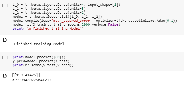
In this case study, we used a simple linear regression problem having one predictor and one label. These same steps and concepts can be extended to more complex multiple linear regression problems(having n number of predictors and one label) as well as classification problems.

I am also sharing my notebook for your reference. In case you get stuck somewhere, feel free to access it from this link:

https://colab.research.google.com/drive/1mDakjr9yQDzc3MDPFimMzqFeC9yvSU4D#scrollTo=u_qOSObBO4H7

TO ADD: Assignment Data for Multiple Linear Regression

I will end this article with a definition of machine learning methodology which I think is easily understandable and generalizable:

In machine learning, instead of writing the algorithm to solve a problem, we use a class of learning methodology (linear regression in this case study) and pass historical data to generate the algorithm, that can be verified and used later to solve the problem.
What is your Definition of machine learning? write in comment.

This was an introduction to machine learning and Tensorflow. If you found this article interesting and want to explore more in this field, you can follow and connect with me.

I will also be adding a few sample assignments and questions to this article later, so keep an eye and bookmark this post. Please share it with others too.

#tensorflow #machine-learning