This is a memo to share what I have learnt in Dimensionality Reduction in Python, capturing the learning objectives as well as my personal notes. The course is taught by Jerone Boeye, and it includes 4 chapters:
Chapter 1. Exploring high dimensional data
Chapter 2. Feature selection I, selecting for feature information
Chapter 3. Feature selection II, selecting for model accuracy
Chapter 4. Feature extraction
Photo by Aditya Chinchure on Unsplash
High-dimensional datasets can be overwhelming and leave you not knowing where to start. Typically, you’d visually explore a new dataset first, but when you have too many dimensions the classical approaches will seem insufficient. Fortunately, there are visualization techniques designed specifically for high dimensional data and you’ll be introduced to these in this course.
After exploring the data, you’ll often find that many features hold little information because they don’t show any variance or because they are duplicates of other features. You’ll learn how to detect these features and drop them from the dataset so that you can focus on the informative ones. In a next step, you might want to build a model on these features, and it may turn out that some don’t have any effect on the thing you’re trying to predict. You’ll learn how to detect and drop these irrelevant features too, in order to reduce dimensionality and thus complexity.
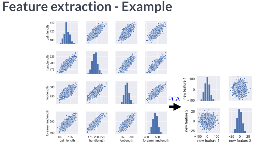
Finally, you’ll learn how feature extraction techniques can reduce dimensionality for you through the calculation of uncorrelated principal components.
Chapter 1. Exploring high dimensional data
You’ll be introduced to the concept of dimensionality reduction and will learn when an why this is important. You’ll learn the difference between feature selection and feature extraction and will apply both techniques for data exploration. The chapter ends with a lesson on t-SNE, a powerful feature extraction technique that will allow you to visualize a high-dimensional dataset.
Introduction
Dataset with more than 10 columns are considered high dimensional data.
Finding the number of dimensions in a dataset
A larger sample of the Pokemon dataset has been loaded for you as the Pandas dataframe pokemon_df.
How many dimensions, or columns are in this dataset?
Answer: 7 dimensions, each Pokemon is described by 7 features.
In [1]: pokemon_df.shape
Out[1]: (160, 7)
Removing features without variance
A sample of the Pokemon dataset has been loaded as pokemon_df. To get an idea of which features have little variance you should use the IPython Shell to calculate summary statistics on this sample. Then adjust the code to create a smaller, easier to understand, dataset.
For the number_cols, Generation column has ‘1’ in all 160 rows.
In [1]: pokemon_df.describe()
Out[1]:
              HP     Attack     Defense  Generation
count  160.00000  160.00000  160.000000       160.0
mean    64.61250   74.98125   70.175000         1.0
std     27.92127   29.18009   28.883533         0.0
min     10.00000    5.00000    5.000000         1.0
25%     45.00000   52.00000   50.000000         1.0
50%     60.00000   71.00000   65.000000         1.0
75%     80.00000   95.00000   85.000000         1.0
max    250.00000  155.00000  180.000000         1.0

# Remove the feature without variance from this list
number_cols = ['HP', 'Attack', 'Defense']
For the non_number_cols, Legendary column has ‘False’ in all 160 rows.
In [6]: pokemon_df[['Name', 'Type', 'Legendary']].describe()
Out[6]:
        Name   Type Legendary
count    160    160       160
unique   160     15         1
top     Abra  Water     False
freq       1     31       160

# Remove the feature without variance from this list
non_number_cols = ['Name', 'Type']
# Create a new dataframe by subselecting the chosen features
df_selected = pokemon_df[number_cols + non_number_cols]
# Prints the first 5 lines of the new dataframe
print(df_selected.head())
<script.py> output:
       HP  Attack  Defense                   Name   Type
    0  45      49       49              Bulbasaur  Grass
    1  60      62       63                Ivysaur  Grass
    2  80      82       83               Venusaur  Grass
    3  80     100      123  VenusaurMega Venusaur  Grass
    4  39      52       43             Charmander   Fire
All Pokemon in this dataset are non-legendary and from generation one so you could choose to drop those two features.
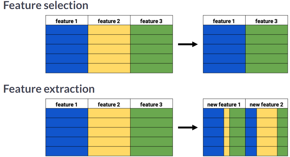
Feature selection vs feature extraction
Why reduce dimensionality?
· dataset will be less complex
· dataset will take up less storage space
· dataset will require less computation time
· dataset will have lower chance of model overfitting
Visually detecting redundant features
Data visualization is a crucial step in any data exploration. Let’s use Seaborn to explore some samples of the US Army ANSUR body measurement dataset.
Two data samples have been pre-loaded as ansur_df_1 and ansur_df_2.
Seaborn has been imported as sns.
# Create a pairplot and color the points using the 'Gender' feature
sns.pairplot(ansur_df_1, hue='Gender', diag_kind='hist')
plt.show()
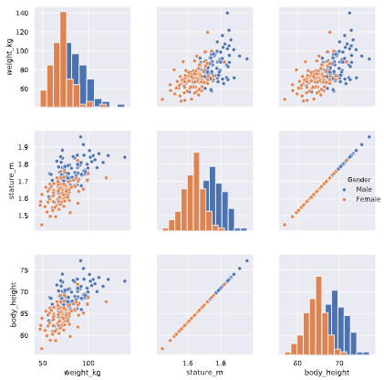
Two features are basically duplicates, remove one of them from the dataset.
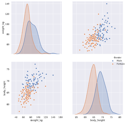
# Remove one of the redundant features
reduced_df = ansur_df_1.drop('stature_m', axis=1)

# Create a pairplot and color the points using the 'Gender' feature
sns.pairplot(reduced_df, hue='Gender')
# Show the plot
plt.show()
# Create a pairplot and color the points using the 'Gender' feature
sns.pairplot(ansur_df_2, hue='Gender', diag_kind='hist')
plt.show()
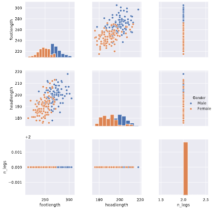
One feature has no variance, remove it from the dataset.
# Remove the redundant feature
reduced_df = ansur_df_2.drop('n_legs', axis=1)

# Create a pairplot and color the points using the 'Gender' feature
sns.pairplot(reduced_df, hue='Gender', diag_kind='hist')
# Show the plot
plt.show()
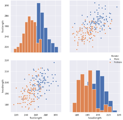
The body height (inches) and stature (meters) hold the same information in a different unit + all the individuals in the second sample have two legs.
Advantage of feature selection
What advantage does feature selection have over feature extraction?
Answer: The selected features remain unchanged, and are therefore easy to interpret.
Extracted features can be quite hard to interpret.
#python #data #dimensionality-reduction