Learn Machine Learning with Python for Absolute Beginners
Machine Learning with Python - Basics
We are living in the ‘age of data’ that is enriched with better computational power and more storage resources,. This data or information is increasing day by day, but the real challenge is to make sense of all the data. Businesses & organizations are trying to deal with it by building intelligent systems using the concepts and methodologies from Data science, Data Mining and Machine learning. Among them, machine learning is the most exciting field of computer science. It would not be wrong if we call machine learning the application and science of algorithms that provides sense to the data.
What is Machine Learning?
Machine Learning (ML) is that field of computer science with the help of which computer systems can provide sense to data in much the same way as human beings do.
In simple words, ML is a type of artificial intelligence that extract patterns out of raw data by using an algorithm or method. The main focus of ML is to allow computer systems learn from experience without being explicitly programmed or human intervention.
Need for Machine Learning
Human beings, at this moment, are the most intelligent and advanced species on earth because they can think, evaluate and solve complex problems. On the other side, AI is still in its initial stage and haven’t surpassed human intelligence in many aspects. Then the question is that what is the need to make machine learn? The most suitable reason for doing this is, “to make decisions, based on data, with efficiency and scale”.
Lately, organizations are investing heavily in newer technologies like Artificial Intelligence, Machine Learning and Deep Learning to get the key information from data to perform several real-world tasks and solve problems. We can call it data-driven decisions taken by machines, particularly to automate the process. These data-driven decisions can be used, instead of using programing logic, in the problems that cannot be programmed inherently. The fact is that we can’t do without human intelligence, but other aspect is that we all need to solve real-world problems with efficiency at a huge scale. That is why the need for machine learning arises.
Why & When to Make Machines Learn?
We have already discussed the need for machine learning, but another question arises that in what scenarios we must make the machine learn? There can be several circumstances where we need machines to take data-driven decisions with efficiency and at a huge scale. The followings are some of such circumstances where making machines learn would be more effective.
Lack of human expertise
The very first scenario in which we want a machine to learn and take data-driven decisions, can be the domain where there is a lack of human expertise. The examples can be navigations in unknown territories or spatial planets.
Dynamic scenarios
There are some scenarios which are dynamic in nature i.e. they keep changing over time. In case of these scenarios and behaviors, we want a machine to learn and take data-driven decisions. Some of the examples can be network connectivity and availability of infrastructure in an organization.
Difficulty in translating expertise into computational tasks
There can be various domains in which humans have their expertise,; however, they are unable to translate this expertise into computational tasks. In such circumstances we want machine learning. The examples can be the domains of speech recognition, cognitive tasks etc.
Machine Learning Model
Before discussing the machine learning model, we must need to understand the following formal definition of ML given by professor Mitchell
“A computer program is said to learn from experience E with respect to some class of tasks T and performance measure P, if its performance at tasks in T, as measured by P, improves with experience E.”
The above definition is basically focusing on three parameters, also the main components of any learning algorithm, namely Task(T), Performance§ and experience (E). In this context, we can simplify this definition as −
ML is a field of AI consisting of learning algorithms that
- Improve their performance §
- At executing some task (T)
- Over time with experience (E)
Based on the above, the following diagram represents a Machine Learning Model
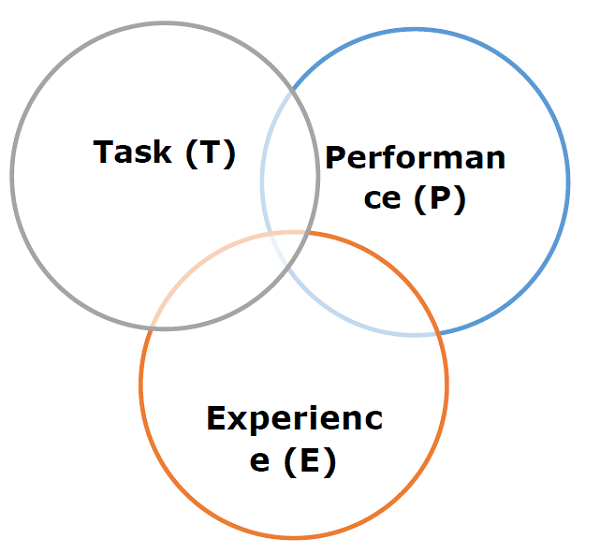
Let us discuss them more in detail now −
Task(T)
From the perspective of problem, we may define the task T as the real-world problem to be solved. The problem can be anything like finding best house price in a specific location or to find best marketing strategy etc. On the other hand, if we talk about machine learning, the definition of task is different because it is difficult to solve ML based tasks by conventional programming approach.
A task T is said to be a ML based task when it is based on the process and the system must follow for operating on data points. The examples of ML based tasks are Classification, Regression, Structured annotation, Clustering, Transcription etc.
Experience (E)
As name suggests, it is the knowledge gained from data points provided to the algorithm or model. Once provided with the dataset, the model will run iteratively and will learn some inherent pattern. The learning thus acquired is called experience(E). Making an analogy with human learning, we can think of this situation as in which a human being is learning or gaining some experience from various attributes like situation, relationships etc. Supervised, unsupervised and reinforcement learning are some ways to learn or gain experience. The experience gained by out ML model or algorithm will be used to solve the task T.
Performance §
An ML algorithm is supposed to perform task and gain experience with the passage of time. The measure which tells whether ML algorithm is performing as per expectation or not is its performance §. P is basically a quantitative metric that tells how a model is performing the task, T, using its experience, E. There are many metrics that help to understand the ML performance, such as accuracy score, F1 score, confusion matrix, precision, recall, sensitivity etc.
Challenges in Machines Learning
While Machine Learning is rapidly evolving, making significant strides with cybersecurity and autonomous cars, this segment of AI as whole still has a long way to go. The reason behind is that ML has not been able to overcome number of challenges. The challenges that ML is facing currently are
Quality of data − Having good-quality data for ML algorithms is one of the biggest challenges. Use of low-quality data leads to the problems related to data preprocessing and feature extraction.
Time-Consuming task − Another challenge faced by ML models is the consumption of time especially for data acquisition, feature extraction and retrieval.
Lack of specialist persons − As ML technology is still in its infancy stage, availability of expert resources is a tough job.
No clear objective for formulating business problems − Having no clear objective and well-defined goal for business problems is another key challenge for ML because this technology is not that mature yet.
Issue of overfitting & underfitting − If the model is overfitting or underfitting, it cannot be represented well for the problem.
Curse of dimensionality − Another challenge ML model faces is too many features of data points. This can be a real hindrance.
Difficulty in deployment − Complexity of the ML model makes it quite difficult to be deployed in real life.
Applications of Machines Learning
Machine Learning is the most rapidly growing technology and according to researchers we are in the golden year of AI and ML. It is used to solve many real-world complex problems which cannot be solved with traditional approach. Following are some real-world applications of ML
- Improve their performance §
- At executing some task (T)
- Over time with experience (E)
Machine Learning with Python - Ecosystem
An Introduction to Python
Python is a popular object-oriented programing language having the capabilities of high-level programming language. Its easy to learn syntax and portability capability makes it popular these days. The followings facts gives us the introduction to Python
- Improve their performance §
- At executing some task (T)
- Over time with experience (E)
Strengths and Weaknesses of Python
Every programming language has some strengths as well as weaknesses, so does Python too.
Strengths
According to studies and surveys, Python is the fifth most important language as well as the most popular language for machine learning and data science. It is because of the following strengths that Python has −
Easy to learn and understand − The syntax of Python is simpler; hence it is relatively easy, even for beginners also, to learn and understand the language.
Multi-purpose language − Python is a multi-purpose programming language because it supports structured programming, object-oriented programming as well as functional programming.
Huge number of modules − Python has huge number of modules for covering every aspect of programming. These modules are easily available for use hence making Python an extensible language.
Support of open source community − As being open source programming language, Python is supported by a very large developer community. Due to this, the bugs are easily fixed by the Python community. This characteristic makes Python very robust and adaptive.
Scalability − Python is a scalable programming language because it provides an improved structure for supporting large programs than shell-scripts.
Weakness
Although Python is a popular and powerful programming language, it has its own weakness of slow execution speed.
The execution speed of Python is slow as compared to compiled languages because Python is an interpreted language. This can be the major area of improvement for Python community.
Installing Python
For working in Python, we must first have to install it. You can perform the installation of Python in any of the following two ways
- Improve their performance §
- At executing some task (T)
- Over time with experience (E)
Let us discuss these each in detail.
Installing Python Individually
If you want to install Python on your computer, then then you need to download only the binary code applicable for your platform. Python distribution is available for Windows, Linux and Mac platforms.
The following is a quick overview of installing Python on the above-mentioned platforms −
On Unix and Linux platform
With the help of following steps, we can install Python on Unix and Linux platform −
- Improve their performance §
- At executing some task (T)
- Over time with experience (E)
On Windows platform
With the help of following steps, we can install Python on Windows platform −
- Improve their performance §
- At executing some task (T)
- Over time with experience (E)
On Macintosh platform
For Mac OS X, Homebrew, a great and easy to use package installer is recommended to install Python 3. In case if you don’t have Homebrew, you can install it with the help of following command −
$ ruby -e "$(curl -fsSL https://raw.githubusercontent.com/Homebrew/install/master/install)"
It can be updated with the command below
$ brew update
Now, to install Python3 on your system, we need to run the following command −
$ brew install python3
Using Pre-packaged Python Distribution: Anaconda
Anaconda is a packaged compilation of Python which have all the libraries widely used in Data science. We can follow the following steps to setup Python environment using Anaconda −
- Improve their performance §
- At executing some task (T)
- Over time with experience (E)
Why Python for Data Science?
Python is the fifth most important language as well as most popular language for Machine learning and data science. The following are the features of Python that makes it the preferred choice of language for data science −
Extensive set of packages
Python has an extensive and powerful set of packages which are ready to be used in various domains. It also has packages like numpy, scipy, pandas, scikit-learn etc. which are required for machine learning and data science.
Easy prototyping
Another important feature of Python that makes it the choice of language for data science is the easy and fast prototyping. This feature is useful for developing new algorithm.
Collaboration feature
The field of data science basically needs good collaboration and Python provides many useful tools that make this extremely.
One language for many domains
A typical data science project includes various domains like data extraction, data manipulation, data analysis, feature extraction, modelling, evaluation, deployment and updating the solution. As Python is a multi-purpose language, it allows the data scientist to address all these domains from a common platform.
Components of Python ML Ecosystem
In this section, let us discuss some core Data Science libraries that form the components of Python Machine learning ecosystem. These useful components make Python an important language for Data Science. Though there are many such components, let us discuss some of the importance components of Python ecosystem here
- Improve their performance §
- At executing some task (T)
- Over time with experience (E)
Machine Learning with Python - Methods
There are various ML algorithms, techniques and methods that can be used to build models for solving real-life problems by using data. In this chapter, we are going to discuss such different kinds of methods.
Different Types of Methods
The following are various ML methods based on some broad categories
- Improve their performance §
- At executing some task (T)
- Over time with experience (E)
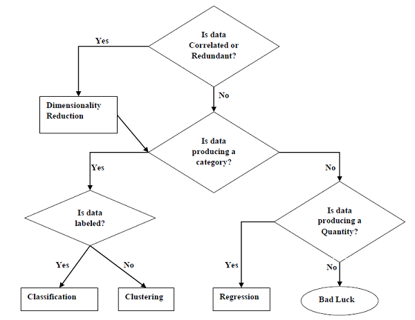
Tasks Suited for Machine Learning
The following diagram shows what type of task is appropriate for various ML problems
Based on learning ability
In the learning process, the following are some methods that are based on learning ability −
Batch Learning
In many cases, we have end-to-end Machine Learning systems in which we need to train the model in one go by using whole available training data. Such kind of learning method or algorithm is called Batch or Offline learning. It is called Batch or Offline learning because it is a one-time procedure and the model will be trained with data in one single batch. The following are the main steps of Batch learning methods −
- Improve their performance §
- At executing some task (T)
- Over time with experience (E)
Online Learning
It is completely opposite to the batch or offline learning methods. In these learning methods, the training data is supplied in multiple incremental batches, called mini-batches, to the algorithm. Followings are the main steps of Online learning methods
- Improve their performance §
- At executing some task (T)
- Over time with experience (E)
Based on Generalization Approach
In the learning process, followings are some methods that are based on generalization approaches −
Instance based Learning
Instance based learning method is one of the useful methods that build the ML models by doing generalization based on the input data. It is opposite to the previously studied learning methods in the way that this kind of learning involves ML systems as well as methods that uses the raw data points themselves to draw the outcomes for newer data samples without building an explicit model on training data.
In simple words, instance-based learning basically starts working by looking at the input data points and then using a similarity metric, it will generalize and predict the new data points.
Model based Learning
In Model based learning methods, an iterative process takes place on the ML models that are built based on various model parameters, called hyperparameters and in which input data is used to extract the features. In this learning, hyperparameters are optimized based on various model validation techniques. That is why we can say that Model based learning methods uses more traditional ML approach towards generalization.
Data Loading for ML Projects
Suppose if you want to start a ML project then what is the first and most important thing you would require? It is the data that we need to load for starting any of the ML project. With respect to data, the most common format of data for ML projects is CSV (comma-separated values).
Basically, CSV is a simple file format which is used to store tabular data (number and text) such as a spreadsheet in plain text. In Python, we can load CSV data into with different ways but before loading CSV data we must have to take care about some considerations.
Consideration While Loading CSV data
CSV data format is the most common format for ML data, but we need to take care about following major considerations while loading the same into our ML projects.
File Header
In CSV data files, the header contains the information for each field. We must use the same delimiter for the header file and for data file because it is the header file that specifies how should data fields be interpreted.
The following are the two cases related to CSV file header which must be considered
- Improve their performance §
- At executing some task (T)
- Over time with experience (E)
In both the cases, we must need to specify explicitly weather our CSV file contains header or not.
Comments
Comments in any data file are having their significance. In CSV data file, comments are indicated by a hash (#) at the start of the line. We need to consider comments while loading CSV data into ML projects because if we are having comments in the file then we may need to indicate, depends upon the method we choose for loading, whether to expect those comments or not.
Delimiter
In CSV data files, comma (,) character is the standard delimiter. The role of delimiter is to separate the values in the fields. It is important to consider the role of delimiter while uploading the CSV file into ML projects because we can also use a different delimiter such as a tab or white space. But in the case of using a different delimiter than standard one, we must have to specify it explicitly.
Quotes
In CSV data files, double quotation (“ ”) mark is the default quote character. It is important to consider the role of quotes while uploading the CSV file into ML projects because we can also use other quote character than double quotation mark. But in case of using a different quote character than standard one, we must have to specify it explicitly.
Methods to Load CSV Data File
While working with ML projects, the most crucial task is to load the data properly into it. The most common data format for ML projects is CSV and it comes in various flavors and varying difficulties to parse. In this section, we are going to discuss about three common approaches in Python to load CSV data file −
Load CSV with Python Standard Library
The first and most used approach to load CSV data file is the use of Python standard library which provides us a variety of built-in modules namely csv module and the reader()function. The following is an example of loading CSV data file with the help of it
Example
In this example, we are using the iris flower data set which can be downloaded into our local directory. After loading the data file, we can convert it into
array and use it for ML projects. Following is the Python script for loading CSV data file
First, we need to import the csv module provided by Python standard library as follows
import csv
Next, we need to import Numpy module for converting the loaded data into NumPy array.
import numpy as np
Now, provide the full path of the file, stored on our local directory, having the CSV data file
path = r"c:\iris.csv"
Next, use the csv.reader()function to read data from CSV file
with open(path,'r') as f:
reader = csv.reader(f,delimiter = ',')
headers = next(reader)
data = list(reader)
data = np.array(data).astype(float)
We can print the names of the headers with the following line of script
print(headers)
The following line of script will print the shape of the data i.e. number of rows & columns in the file
print(data.shape)
Next script line will give the first three line of data file
print(data[:3])
Output
['sepal_length', 'sepal_width', 'petal_length', 'petal_width']
(150, 4)
[[5.1 3.5 1.4 0.2]
[4.9 3. 1.4 0.2]
[4.7 3.2 1.3 0.2]]
Load CSV with NumPy
Another approach to load CSV data file is NumPy and numpy.loadtxt() function. The following is an example of loading CSV data file with the help of it
Example
In this example, we are using the Pima Indians Dataset having the data of diabetic patients. This dataset is a numeric dataset with no header. It can also be downloaded into our local directory. After loading the data file, we can convert it into NumPy array and use it for ML projects. The following is the Python script for loading CSV data file
from numpy import loadtxt
path = r"C:\pima-indians-diabetes.csv"
datapath= open(path, 'r')
data = loadtxt(datapath, delimiter=",")
print(data.shape)
print(data[:3])
Output
(768, 9)
[[ 6. 148. 72. 35. 0. 33.6 0.627 50. 1.]
[ 1. 85. 66. 29. 0. 26.6 0.351 31. 0.]
[ 8. 183. 64. 0. 0. 23.3 0.672 32. 1.]]
Load CSV with Pandas
Another approach to load CSV data file is by Pandas and pandas.read_csv()function. This is the very flexible function that returns a pandas.DataFrame which can be used immediately for plotting. The following is an example of loading CSV data file with the help of it
Example
Here, we will be implementing two Python scripts, first is with Iris data set having headers and another is by using the Pima Indians Dataset which is a numeric dataset with no header. Both the datasets can be downloaded into local directory.
Script-1
The following is the Python script for loading CSV data file using Pandas on Iris Data set
from pandas import read_csv
path = r"C:\iris.csv"
data = read_csv(path)
print(data.shape)
print(data[:3])
Output
(150, 4)
sepal_length sepal_width petal_length petal_width
0 5.1       3.5        1.4         0.2
1 4.9       3.0        1.4         0.2
2 4.7       3.2        1.3         0.2
Script-2
The following is the Python script for loading CSV data file, along with providing the headers names too, using Pandas on Pima Indians Diabetes dataset
from pandas import read_csv
path = r"C:\pima-indians-diabetes.csv"
headernames = ['preg', 'plas', 'pres', 'skin', 'test', 'mass', 'pedi', 'age', 'class']
data = read_csv(path, names=headernames)
print(data.shape)
print(data[:3])
Output
(768, 9)
  preg plas   pres skin test mass  pedi age class
0    6  148     72   35    0 33.6 0.627  50     1
1    1   85     66   29    0 26.6 0.351  31     0
2    8  183     64    0    0 23.3 0.672  32     1
The difference between above used three approaches for loading CSV data file can easily be understood with the help of given examples.
ML - Understanding Data with Statistics
Introduction
While working with machine learning projects, usually we ignore two most important parts called mathematics and data. It is because, we know that ML is a data driven approach and our ML model will produce only as good or as bad results as the data we provided to it.
In the previous chapter, we discussed how we can upload CSV data into our ML project, but it would be good to understand the data before uploading it. We can understand the data by two ways, with statistics and with visualization.
In this chapter, with the help of following Python recipes, we are going to understand ML data with statistics.
Looking at Raw Data
The very first recipe is for looking at your raw data. It is important to look at raw data because the insight we will get after looking at raw data will boost our chances to better pre-processing as well as handling of data for ML projects.
Following is a Python script implemented by using head() function of Pandas DataFrame on Pima Indians diabetes dataset to look at the first 50 rows to get better understanding of it
Example
from pandas import read_csv
path = r"C:\pima-indians-diabetes.csv"
headernames = ['preg', 'plas', 'pres', 'skin', 'test', 'mass', 'pedi', 'age', 'class']
data = read_csv(path, names=headernames)
print(data.head(50))
Output
preg plas pres skin test  mass pedi  age     class
0    6   148 72  35    0   33.6  0.627   50    1
1    1    85 66  29    0   26.6  0.351   31    0
2    8   183 64   0    0   23.3  0.672   32    1
3    1    89 66  23   94   28.1  0.167   21    0
4    0   137 40  35  168   43.1  2.288   33    1
5    5   116 74   0    0   25.6  0.201   30    0
6    3    78 50  32   88   31.0  0.248   26    1
7   10   115  0   0    0   35.3  0.134   29    0
8    2   197 70  45  543   30.5  0.158   53    1
9    8   125 96   0    0    0.0  0.232   54    1
10   4   110 92   0    0   37.6  0.191   30    0
11  10   168 74   0    0   38.0  0.537   34    1
12  10   139 80   0    0   27.1  1.441   57    0
13   1   189 60  23  846   30.1  0.398   59    1
14   5   166 72  19  175   25.8  0.587   51    1
15   7   100  0   0    0   30.0  0.484   32    1
16   0   118 84  47  230   45.8  0.551   31    1
17   7   107 74   0    0   29.6  0.254   31    1
18   1   103 30  38   83   43.3  0.183   33    0
19   1   115 70  30   96   34.6  0.529   32    1
20   3   126 88  41  235   39.3  0.704   27    0
21   8    99 84   0    0   35.4  0.388   50    0
22   7   196 90   0    0   39.8  0.451   41    1
23   9   119 80  35    0   29.0  0.263   29    1
24  11   143 94  33  146   36.6  0.254   51    1
25  10   125 70  26  115   31.1  0.205   41    1
26   7   147 76   0    0   39.4  0.257   43    1
27   1    97 66  15  140   23.2  0.487   22    0
28  13   145 82  19  110   22.2  0.245   57    0
29   5   117 92   0    0   34.1  0.337   38    0
30   5   109 75  26    0   36.0  0.546   60    0
31   3   158 76  36  245   31.6  0.851   28    1
32   3    88 58  11   54   24.8  0.267   22    0
33   6    92 92   0    0   19.9  0.188   28    0
34  10   122 78   31    0   27.6  0.512   45    0
35   4   103 60  33  192   24.0  0.966   33    0
36  11   138 76   0    0   33.2  0.420   35    0
37   9   102 76  37    0   32.9  0.665   46    1
38   2    90 68  42    0   38.2  0.503   27    1
39   4   111 72  47  207   37.1  1.390   56    1
40   3   180 64  25   70   34.0  0.271   26    0
41   7   133 84   0    0   40.2  0.696   37    0
42   7   106 92  18    0   22.7  0.235   48    0
43   9    171 110  24  240   45.4  0.721   54    1
44   7   159 64   0    0   27.4  0.294   40    0
45   0   180 66  39    0   42.0  1.893   25    1
46   1   146 56   0    0   29.7  0.564   29    0
47   2    71 70  27    0   28.0  0.586   22    0
48   7   103 66  32    0   39.1  0.344   31    1
49   7   105  0   0    0   0.0   0.305   24    0
We can observe from the above output that first column gives the row number which can be very useful for referencing a specific observation.
Checking Dimensions of Data
It is always a good practice to know how much data, in terms of rows and columns, we are having for our ML project. The reasons behind are
- Improve their performance §
- At executing some task (T)
- Over time with experience (E)
Following is a Python script implemented by printing the shape property on Pandas Data Frame. We are going to implement it on iris data set for getting the total number of rows and columns in it.
Example
from pandas import read_csv
path = r"C:\iris.csv"
data = read_csv(path)
print(data.shape)
Output
(150, 4)
We can easily observe from the output that iris data set, we are going to use, is having 150 rows and 4 columns.
Getting Each Attribute’s Data Type
It is another good practice to know data type of each attribute. The reason behind is that, as per to the requirement, sometimes we may need to convert one data type to another. For example, we may need to convert string into floating point or int for representing categorial or ordinal values. We can have an idea about the attribute’s data type by looking at the raw data, but another way is to use dtypes property of Pandas DataFrame. With the help of dtypes property we can categorize each attributes data type. It can be understood with the help of following Python script
Example
from pandas import read_csv
path = r"C:\iris.csv"
data = read_csv(path)
print(data.dtypes)
Output
sepal_length  float64
sepal_width   float64
petal_length  float64
petal_width   float64
dtype: object
From the above output, we can easily get the datatypes of each attribute.
Statistical Summary of Data
We have discussed Python recipe to get the shape i.e. number of rows and columns, of data but many times we need to review the summaries out of that shape of data. It can be done with the help of describe() function of Pandas DataFrame that further provide the following 8 statistical properties of each & every data attribute −
- Improve their performance §
- At executing some task (T)
- Over time with experience (E)
Example
from pandas import read_csv
from pandas import set_option
path = r"C:\pima-indians-diabetes.csv"
names = ['preg', 'plas', 'pres', 'skin', 'test', 'mass', 'pedi', 'age', 'class']
data = read_csv(path, names=names)
set_option('display.width', 100)
set_option('precision', 2)
print(data.shape)
print(data.describe())
Output
(768, 9)
      preg    plas    pres   skin    test    mass    pedi    age     class
count 768.00  768.00  768.00 768.00  768.00  768.00  768.00  768.00  768.00
mean    3.85  120.89   69.11  20.54   79.80   31.99    0.47   33.24    0.35
std     3.37   31.97   19.36  15.95  115.24    7.88    0.33   11.76    0.48
min     0.00    0.00    0.00   0.00    0.00    0.00    0.08   21.00    0.00
25%     1.00   99.00   62.00   0.00    0.00   27.30    0.24   24.00    0.00
50%     3.00  117.00   72.00  23.00   30.50   32.00    0.37   29.00    0.00
75%     6.00  140.25   80.00  32.00  127.25   36.60    0.63   41.00    1.00
max    17.00  199.00  122.00  99.00  846.00   67.10    2.42   81.00    1.00
From the above output, we can observe the statistical summary of the data of Pima Indian Diabetes dataset along with shape of data.
Reviewing Class Distribution
Class distribution statistics is useful in classification problems where we need to know the balance of class values. It is important to know class value distribution because if we have highly imbalanced class distribution i.e. one class is having lots more observations than other class, then it may need special handling at data preparation stage of our ML project. We can easily get class distribution in Python with the help of Pandas DataFrame.
Example
from pandas import read_csv
path = r"C:\pima-indians-diabetes.csv"
names = ['preg', 'plas', 'pres', 'skin', 'test', 'mass', 'pedi', 'age', 'class']
data = read_csv(path, names=names)
count_class = data.groupby('class').size()
print(count_class)
Output
Class
0 500
1 268
dtype: int64
From the above output, it can be clearly seen that the number of observations with class 0 are almost double than number of observations with class 1.
Reviewing Correlation between Attributes
The relationship between two variables is called correlation. In statistics, the most common method for calculating correlation is Pearson’s Correlation Coefficient. It can have three values as follows −
- Improve their performance §
- At executing some task (T)
- Over time with experience (E)
It is always good for us to review the pairwise correlations of the attributes in our dataset before using it into ML project because some machine learning algorithms such as linear regression and logistic regression will perform poorly if we have highly correlated attributes. In Python, we can easily calculate a correlation matrix of dataset attributes with the help of corr() function on Pandas DataFrame.
Example
from pandas import read_csv
from pandas import set_option
path = r"C:\pima-indians-diabetes.csv"
names = ['preg', 'plas', 'pres', 'skin', 'test', 'mass', 'pedi', 'age', 'class']
data = read_csv(path, names=names)
set_option('display.width', 100)
set_option('precision', 2)
correlations = data.corr(method='pearson')
print(correlations)
Output
preg  plas  pres  skin  test   mass   pedi   age   class
preg  1.00  0.13  0.14 -0.08  -0.07   0.02  -0.03  0.54   0.22
plas  0.13  1.00  0.15  0.06   0.33   0.22   0.14  0.26   0.47
pres  0.14  0.15  1.00  0.21   0.09   0.28   0.04  0.24   0.07
skin -0.08  0.06  0.21  1.00   0.44   0.39   0.18 -0.11   0.07
test -0.07  0.33  0.09  0.44   1.00   0.20   0.19 -0.04   0.13
mass  0.02  0.22  0.28  0.39   0.20   1.00   0.14  0.04   0.29
pedi -0.03  0.14  0.04  0.18   0.19   0.14   1.00  0.03   0.17
age   0.54  0.26  0.24 -0.11  -0.04   0.04   0.03  1.00   0.24
class 0.22  0.47  0.07  0.07   0.13   0.29   0.17  0.24   1.00
The matrix in above output gives the correlation between all the pairs of the attribute in dataset.
Reviewing Skew of Attribute Distribution
Skewness may be defined as the distribution that is assumed to be Gaussian but appears distorted or shifted in one direction or another, or either to the left or right. Reviewing the skewness of attributes is one of the important tasks due to following reasons −
- Improve their performance §
- At executing some task (T)
- Over time with experience (E)
In Python, we can easily calculate the skew of each attribute by using skew() function on Pandas DataFrame.
Example
from pandas import read_csv
path = r"C:\pima-indians-diabetes.csv"
names = ['preg', 'plas', 'pres', 'skin', 'test', 'mass', 'pedi', 'age', 'class']
data = read_csv(path, names=names)
print(data.skew())
Output
preg  0.90
plas  0.17
pres -1.84
skin  0.11
test  2.27
mass -0.43
pedi  1.92
age   1.13
class 0.64
dtype: float64
From the above output, positive or negative skew can be observed. If the value is closer to zero, then it shows less skew.
ML - Understanding Data with Visualization
Introduction
In the previous chapter, we have discussed the importance of data for Machine Learning algorithms along with some Python recipes to understand the data with statistics. There is another way called Visualization, to understand the data.
With the help of data visualization, we can see how the data looks like and what kind of correlation is held by the attributes of data. It is the fastest way to see if the features correspond to the output. With the help of following Python recipes, we can understand ML data with statistics.
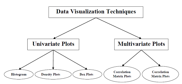
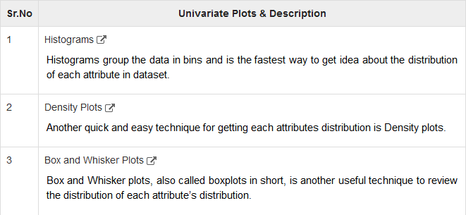
Univariate Plots: Understanding Attributes Independently
The simplest type of visualization is single-variable or “univariate” visualization. With the help of univariate visualization, we can understand each attribute of our dataset independently. The following are some techniques in Python to implement univariate visualization
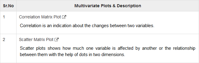
Multivariate Plots: Interaction Among Multiple Variables
Another type of visualization is multi-variable or “multivariate” visualization. With the help of multivariate visualization, we can understand interaction between multiple attributes of our dataset. The following are some techniques in Python to implement multivariate visualization
Machine Learning - Preparing Data
Introduction
Machine Learning algorithms are completely dependent on data because it is the most crucial aspect that makes model training possible. On the other hand, if we won’t be able to make sense out of that data, before feeding it to ML algorithms, a machine will be useless. In simple words, we always need to feed right data i.e. the data in correct scale, format and containing meaningful features, for the problem we want machine to solve.
This makes data preparation the most important step in ML process. Data preparation may be defined as the procedure that makes our dataset more appropriate for ML process.
Why Data Pre-processing?
After selecting the raw data for ML training, the most important task is data pre-processing. In broad sense, data preprocessing will convert the selected data into a form we can work with or can feed to ML algorithms. We always need to preprocess our data so that it can be as per the expectation of machine learning algorithm.
Data Pre-processing Techniques
We have the following data preprocessing techniques that can be applied on data set to produce data for ML algorithms −
Scaling
Most probably our dataset comprises of the attributes with varying scale, but we cannot provide such data to ML algorithm hence it requires rescaling. Data rescaling makes sure that attributes are at same scale. Generally, attributes are rescaled into the range of 0 and 1. ML algorithms like gradient descent and k-Nearest Neighbors requires scaled data. We can rescale the data with the help of MinMaxScaler class of scikit-learn Python library.
Example
In this example we will rescale the data of Pima Indians Diabetes dataset which we used earlier. First, the CSV data will be loaded (as done in the previous chapters) and then with the help of MinMaxScaler class, it will be rescaled in the range of 0 and 1.
The first few lines of the following script are same as we have written in previous chapters while loading CSV data.
from pandas import read_csv
from numpy import set_printoptions
from sklearn import preprocessing
path = r'C:\pima-indians-diabetes.csv'
names = ['preg', 'plas', 'pres', 'skin', 'test', 'mass', 'pedi', 'age', 'class']
dataframe = read_csv(path, names=names)
array = dataframe.values
Now, we can use MinMaxScaler class to rescale the data in the range of 0 and 1.
data_scaler = preprocessing.MinMaxScaler(feature_range=(0,1))
data_rescaled = data_scaler.fit_transform(array)
We can also summarize the data for output as per our choice. Here, we are setting the precision to 1 and showing the first 10 rows in the output.
set_printoptions(precision=1)
print ("\nScaled data:\n", data_rescaled[0:10])
Output
Scaled data:
[[0.4 0.7 0.6 0.4 0. 0.5 0.2 0.5 1. ]
[0.1 0.4 0.5 0.3 0. 0.4 0.1 0.2 0. ]
[0.5 0.9 0.5 0. 0. 0.3 0.3 0.2 1. ]
[0.1 0.4 0.5 0.2 0.1 0.4 0. 0. 0. ]
[0.  0.7 0.3 0.4 0.2 0.6 0.9 0.2 1. ]
[0.3 0.6 0.6 0. 0. 0.4 0.1 0.2 0. ]
[0.2 0.4 0.4 0.3 0.1 0.5 0.1 0.1 1. ]
[0.6 0.6 0. 0. 0. 0.5 0. 0.1 0. ]
[0.1 1. 0.6 0.5 0.6 0.5 0. 0.5 1. ]
[0.5 0.6 0.8 0. 0. 0. 0.1 0.6 1. ]]
From the above output, all the data got rescaled into the range of 0 and 1.
Normalization
Another useful data preprocessing technique is Normalization. This is used to rescale each row of data to have a length of 1. It is mainly useful in Sparse dataset where we have lots of zeros. We can rescale the data with the help of Normalizer class of scikit-learn Python library.
Types of Normalization
In machine learning, there are two types of normalization preprocessing techniques as follows
- Improve their performance §
- At executing some task (T)
- Over time with experience (E)
Binarization
As the name suggests, this is the technique with the help of which we can make our data binary. We can use a binary threshold for making our data binary. The values above that threshold value will be converted to 1 and below that threshold will be converted to 0.
For example, if we choose threshold value = 0.5, then the dataset value above it will become 1 and below this will become 0. That is why we can call it binarizing the data or thresholding the data. This technique is useful when we have probabilities in our dataset and want to convert them into crisp values.
We can binarize the data with the help of Binarizer class of scikit-learn Python library
Example
In this example, we will rescale the data of Pima Indians Diabetes dataset which we used earlier. First, the CSV data will be loaded and then with the help of Binarizer class it will be converted into binary values i.e. 0 and 1 depending upon the threshold value. We are taking 0.5 as threshold value.
The first few lines of following script are same as we have written in previous chapters while loading CSV data.
from pandas import read_csv
from sklearn.preprocessing import Binarizer
path = r'C:\pima-indians-diabetes.csv'
names = ['preg', 'plas', 'pres', 'skin', 'test', 'mass', 'pedi', 'age', 'class']
dataframe = read_csv(path, names=names)
array = dataframe.values
Now, we can use Binarize class to convert the data into binary values.
binarizer = Binarizer(threshold=0.5).fit(array)
Data_binarized = binarizer.transform(array)
Here, we are showing the first 5 rows in the output.
print ("\nBinary data:\n", Data_binarized [0:5])
Output
Binary data:
[[1. 1. 1. 1. 0. 1. 1. 1. 1.]
[1. 1. 1. 1. 0. 1. 0. 1. 0.]
[1. 1. 1. 0. 0. 1. 1. 1. 1.]
[1. 1. 1. 1. 1. 1. 0. 1. 0.]
[0. 1. 1. 1. 1. 1. 1. 1. 1.]]
Standardization
Another useful data preprocessing technique which is basically used to transform the data attributes with a Gaussian distribution. It differs the mean and SD (Standard Deviation) to a standard Gaussian distribution with a mean of 0 and a SD of 1. This technique is useful in ML algorithms like linear regression, logistic regression that assumes a Gaussian distribution in input dataset and produce better results with rescaled data. We can standardize the data (mean = 0 and SD =1) with the help of StandardScaler class of scikit-learn Python library.
Example
In this example, we will rescale the data of Pima Indians Diabetes dataset which we used earlier. First, the CSV data will be loaded and then with the help of StandardScaler class it will be converted into Gaussian Distribution with mean = 0 and SD = 1.
The first few lines of following script are same as we have written in previous chapters while loading CSV data.
from sklearn.preprocessing import StandardScaler
from pandas import read_csv
from numpy import set_printoptions
path = r'C:\pima-indians-diabetes.csv'
names = ['preg', 'plas', 'pres', 'skin', 'test', 'mass', 'pedi', 'age', 'class']
dataframe = read_csv(path, names=names)
array = dataframe.values
Now, we can use StandardScaler class to rescale the data.
data_scaler = StandardScaler().fit(array)
data_rescaled = data_scaler.transform(array)
We can also summarize the data for output as per our choice. Here, we are setting the precision to 2 and showing the first 5 rows in the output.
set_printoptions(precision=2)
print ("\nRescaled data:\n", data_rescaled [0:5])
Output
Rescaled data:
[[ 0.64 0.85 0.15 0.91 -0.69 0.2  0.47 1.43 1.37]
[-0.84 -1.12 -0.16 0.53 -0.69 -0.68 -0.37 -0.19 -0.73]
[ 1.23 1.94 -0.26 -1.29 -0.69 -1.1  0.6 -0.11 1.37]
[-0.84 -1.  -0.16 0.15 0.12 -0.49 -0.92 -1.04 -0.73]
[-1.14 0.5 -1.5  0.91 0.77 1.41 5.48 -0.02 1.37]]
Data Labeling
We discussed the importance of good fata for ML algorithms as well as some techniques to pre-process the data before sending it to ML algorithms. One more aspect in this regard is data labeling. It is also very important to send the data to ML algorithms having proper labeling. For example, in case of classification problems, lot of labels in the form of words, numbers etc. are there on the data.
What is Label Encoding?
Most of the sklearn functions expect that the data with number labels rather than word labels. Hence, we need to convert such labels into number labels. This process is called label encoding. We can perform label encoding of data with the help of LabelEncoder() function of scikit-learn Python library.
Example
In the following example, Python script will perform the label encoding.
First, import the required Python libraries as follows
import numpy as np
from sklearn import preprocessing
Now, we need to provide the input labels as follows
input_labels = ['red','black','red','green','black','yellow','white']
The next line of code will create the label encoder and train it.
encoder = preprocessing.LabelEncoder()
encoder.fit(input_labels)
The next lines of script will check the performance by encoding the random ordered list
test_labels = ['green','red','black']
encoded_values = encoder.transform(test_labels)
print("\nLabels =", test_labels)
print("Encoded values =", list(encoded_values))
encoded_values = [3,0,4,1]
decoded_list = encoder.inverse_transform(encoded_values)
We can get the list of encoded values with the help of following python script −
print("\nEncoded values =", encoded_values)
print("\nDecoded labels =", list(decoded_list))
Output
Labels = ['green', 'red', 'black']
Encoded values = [1, 2, 0]
Encoded values = [3, 0, 4, 1]
Decoded labels = ['white', 'black', 'yellow', 'green']
Machine Learning - Data Feature Selection
In the previous chapter, we have seen in detail how to preprocess and prepare data for machine learning. In this chapter, let us understand in detail data feature selection and various aspects involved in it.
Importance of Data Feature Selection
The performance of machine learning model is directly proportional to the data features used to train it. The performance of ML model will be affected negatively if the data features provided to it are irrelevant. On the other hand, use of relevant data features can increase the accuracy of your ML model especially linear and logistic regression.
Now the question arise that what is automatic feature selection? It may be defined as the process with the help of which we select those features in our data that are most relevant to the output or prediction variable in which we are interested. It is also called attribute selection.
The following are some of the benefits of automatic feature selection before modeling the data
- Improve their performance §
- At executing some task (T)
- Over time with experience (E)
Feature Selection Techniques
The followings are automatic feature selection techniques that we can use to model ML data in Python
Univariate Selection
This feature selection technique is very useful in selecting those features, with the help of statistical testing, having strongest relationship with the prediction variables. We can implement univariate feature selection technique with the help of SelectKBest0class of scikit-learn Python library.
Example
In this example, we will use Pima Indians Diabetes dataset to select 4 of the attributes having best features with the help of chi-square statistical test.
from pandas import read_csv
from numpy import set_printoptions
from sklearn.feature_selection import SelectKBest
from sklearn.feature_selection import chi2
path = r'C:\pima-indians-diabetes.csv'
names = ['preg', 'plas', 'pres', 'skin', 'test', 'mass', 'pedi', 'age', 'class']
dataframe = read_csv(path, names=names)
array = dataframe.values
Next, we will separate array into input and output components
X = array[:,0:8]
Y = array[:,8]
The following lines of code will select the best features from dataset
test = SelectKBest(score_func=chi2, k=4)
fit = test.fit(X,Y)
We can also summarize the data for output as per our choice. Here, we are setting the precision to 2 and showing the 4 data attributes with best features along with best score of each attribute
set_printoptions(precision=2)
print(fit.scores_)
featured_data = fit.transform(X)
print ("\nFeatured data:\n", featured_data[0:4])
Output
[ 111.52 1411.89 17.61 53.11 2175.57 127.67 5.39 181.3 ]
Featured data:
[[148. 0. 33.6 50. ]
[ 85. 0. 26.6 31. ]
[ 183. 0. 23.3 32. ]
[ 89. 94. 28.1 21. ]]
Recursive Feature Elimination
As the name suggests, RFE (Recursive feature elimination) feature selection technique removes the attributes recursively and builds the model with remaining attributes. We can implement RFE feature selection technique with the help of RFE class of scikit-learn Python library.
Example
In this example, we will use RFE with logistic regression algorithm to select the best 3 attributes having the best features from Pima Indians Diabetes dataset to.
from pandas import read_csv
from sklearn.feature_selection import RFE
from sklearn.linear_model import LogisticRegression
path = r'C:\pima-indians-diabetes.csv'
names = ['preg', 'plas', 'pres', 'skin', 'test', 'mass', 'pedi', 'age', 'class']
dataframe = read_csv(path, names=names)
array = dataframe.values
Next, we will separate the array into its input and output components −
X = array[:,0:8]
Y = array[:,8]
The following lines of code will select the best features from a dataset
model = LogisticRegression()
rfe = RFE(model, 3)
fit = rfe.fit(X, Y)
print("Number of Features: %d")
print("Selected Features: %s")
print("Feature Ranking: %s")
Output
Number of Features: 3
Selected Features: [ True False False False False True True False]
Feature Ranking: [1 2 3 5 6 1 1 4]
We can see in above output, RFE choose preg, mass and pedi as the first 3 best features. They are marked as 1 in the output.
Principal Component Analysis (PCA)
PCA, generally called data reduction technique, is very useful feature selection technique as it uses linear algebra to transform the dataset into a compressed form. We can implement PCA feature selection technique with the help of PCA class of scikit-learn Python library. We can select number of principal components in the output.
Example
In this example, we will use PCA to select best 3 Principal components from Pima Indians Diabetes dataset.
from pandas import read_csv
from sklearn.decomposition import PCA
path = r'C:\pima-indians-diabetes.csv'
names = ['preg', 'plas', 'pres', 'skin', 'test', 'mass', 'pedi', 'age', 'class']
dataframe = read_csv(path, names=names)
array = dataframe.values
Next, we will separate array into input and output components −
X = array[:,0:8]
Y = array[:,8]
The following lines of code will extract features from dataset
pca = PCA(n_components = 3)
fit = pca.fit(X)
print("Explained Variance: %s") % fit.explained_variance_ratio_
print(fit.components_)
Output
Explained Variance: [ 0.88854663 0.06159078 0.02579012]
[[ -2.02176587e-03 9.78115765e-02 1.60930503e-02 6.07566861e-02
9.93110844e-01 1.40108085e-02 5.37167919e-04 -3.56474430e-03]
[ 2.26488861e-02 9.72210040e-01 1.41909330e-01 -5.78614699e-02
-9.46266913e-02 4.69729766e-02 8.16804621e-04 1.40168181e-01]
[ -2.24649003e-02 1.43428710e-01 -9.22467192e-01 -3.07013055e-01
2.09773019e-02 -1.32444542e-01 -6.39983017e-04 -1.25454310e-01]]
We can observe from the above output that 3 Principal Components bear little resemblance to the source data.
Feature Importance
As the name suggests, feature importance technique is used to choose the importance features. It basically uses a trained supervised classifier to select features. We can implement this feature selection technique with the help of ExtraTreeClassifier class of scikit-learn Python library.
Example
In this example, we will use ExtraTreeClassifier to select features from Pima Indians Diabetes dataset.
from pandas import read_csv
from sklearn.ensemble import ExtraTreesClassifier
path = r'C:\Desktop\pima-indians-diabetes.csv'
names = ['preg', 'plas', 'pres', 'skin', 'test', 'mass', 'pedi', 'age', 'class']
dataframe = read_csv(data, names=names)
array = dataframe.values
Next, we will separate array into input and output components
X = array[:,0:8]
Y = array[:,8]
The following lines of code will extract features from dataset
model = ExtraTreesClassifier()
model.fit(X, Y)
print(model.feature_importances_)
Output
[ 0.11070069 0.2213717 0.08824115 0.08068703 0.07281761 0.14548537 0.12654214 0.15415431]
From the output, we can observe that there are scores for each attribute. The higher the score, higher is the importance of that attribute.
Classification Algorithms - Introduction
Introduction to Classification
Classification may be defined as the process of predicting class or category from observed values or given data points. The categorized output can have the form such as “Black” or “White” or “spam” or “no spam”.
Mathematically, classification is the task of approximating a mapping function (f) from input variables (X) to output variables (Y). It is basically belongs to the supervised machine learning in which targets are also provided along with the input data set.
An example of classification problem can be the spam detection in emails. There can be only two categories of output, “spam” and “no spam”; hence this is a binary type classification.
To implement this classification, we first need to train the classifier. For this example, “spam” and “no spam” emails would be used as the training data. After successfully train the classifier, it can be used to detect an unknown email.
Types of Learners in Classification
We have two types of learners in respective to classification problems −
Lazy Learners
As the name suggests, such kind of learners waits for the testing data to be appeared after storing the training data. Classification is done only after getting the testing data. They spend less time on training but more time on predicting. Examples of lazy learners are K-nearest neighbor and case-based reasoning.
Eager Learners
As opposite to lazy learners, eager learners construct classification model without waiting for the testing data to be appeared after storing the training data. They spend more time on training but less time on predicting. Examples of eager learners are Decision Trees, Naïve Bayes and Artificial Neural Networks (ANN).
Building a Classifier in Python
Scikit-learn, a Python library for machine learning can be used to build a classifier in Python. The steps for building a classifier in Python are as follows
Step 1: Importing necessary python package
For building a classifier using scikit-learn, we need to import it. We can import it by using following script
import sklearn
Step 2: Importing dataset
After importing necessary package, we need a dataset to build classification prediction model. We can import it from sklearn dataset or can use other one as per our requirement. We are going to use sklearn’s Breast Cancer Wisconsin Diagnostic Database. We can import it with the help of following script
from sklearn.datasets import load_breast_cancer
The following script will load the dataset;
data = load_breast_cancer()
We also need to organize the data and it can be done with the help of following scripts
label_names = data['target_names']
labels = data['target']
feature_names = data['feature_names']
features = data['data']
The following command will print the name of the labels, ‘malignant’ and ‘benign’ in case of our database.
print(label_names)
The output of the above command is the names of the labels
['malignant' 'benign']
These labels are mapped to binary values 0 and 1. Malignant cancer is represented by 0 and Benign cancer is represented by 1.
The feature names and feature values of these labels can be seen with the help of following commands
print(feature_names[0])
The output of the above command is the names of the features for label 0 i.e. Malignant cancer
mean radius
Similarly, names of the features for label can be produced as follows
print(feature_names[1])
The output of the above command is the names of the features for label 1 i.e. Benign cancer
mean texture
We can print the features for these labels with the help of following command
print(features[0])
This will give the following output
[1.799e+01 1.038e+01 1.228e+02 1.001e+03 1.184e-01 2.776e-01 3.001e-01
 1.471e-01 2.419e-01 7.871e-02 1.095e+00 9.053e-01 8.589e+00 1.534e+02
 6.399e-03 4.904e-02 5.373e-02 1.587e-02 3.003e-02 6.193e-03 2.538e+01
 1.733e+01 1.846e+02 2.019e+03 1.622e-01 6.656e-01 7.119e-01 2.654e-01
 4.601e-01 1.189e-01]
We can print the features for these labels with the help of following command
print(features[1])
This will give the following output
[2.057e+01 1.777e+01 1.329e+02 1.326e+03 8.474e-02 7.864e-02 8.690e-02
7.017e-02 1.812e-01 5.667e-02 5.435e-01 7.339e-01 3.398e+00 7.408e+01
5.225e-03 1.308e-02 1.860e-02 1.340e-02 1.389e-02 3.532e-03 2.499e+01
2.341e+01 1.588e+02 1.956e+03 1.238e-01 1.866e-01 2.416e-01 1.860e-01
2.750e-01 8.902e-02]
Step 3: Organizing data into training & testing sets
As we need to test our model on unseen data, we will divide our dataset into two parts: a training set and a test set. We can use train_test_split() function of sklearn python package to split the data into sets. The following command will import the function
from sklearn.model_selection import train_test_split
Now, next command will split the data into training & testing data. In this example, we are using taking 40 percent of the data for testing purpose and 60 percent of the data for training purpose
train, test, train_labels, test_labels =
  train_test_split(features,labels,test_size = 0.40, random_state = 42)
Step 4: Model evaluation
After dividing the data into training and testing we need to build the model. We will be using Naïve Bayes algorithm for this purpose. The following commands will import the GaussianNB module
from sklearn.naive_bayes import GaussianNB
Now, initialize the model as follows
gnb = GaussianNB()
Next, with the help of following command we can train the model
model = gnb.fit(train, train_labels)
Now, for evaluation purpose we need to make predictions. It can be done by using predict() function as follows
preds = gnb.predict(test)
print(preds)
This will give the following output −
[1 0 0 1 1 0 0 0 1 1 1 0 1 0 1 0 1 1 1 0 1 1 0 1 1 1 1 1 1 0 1 1 1 1 1 1 0
 1 0 1 1 0 1 1 1 1 1 1 1 1 0 0 1 1 1 1 1 0 0 1 1 0 0 1 1 1 0 0 1 1 0 0 1 0
 1 1 1 1 1 1 0 1 1 0 0 0 0 0 1 1 1 1 1 1 1 1 0 0 1 0 0 1 0 0 1 1 1 0 1 1 0
 1 1 0 0 0 1 1 1 0 0 1 1 0 1 0 0 1 1 0 0 0 1 1 1 0 1 1 0 0 1 0 1 1 0 1 0 0
 1 1 1 1 1 1 1 0 0 1 1 1 1 1 1 1 1 1 1 1 1 0 1 1 1 0 1 1 0 1 1 1 1 1 1 0 0
 0 1 1 0 1 0 1 1 1 1 0 1 1 0 1 1 1 0 1 0 0 1 1 1 1 1 1 1 1 0 1 1 1 1 1 0 1
 0 0 1 1 0 1]
The above series of 0s and 1s in output are the predicted values for the Malignant and Benign tumor classes.
Step 5: Finding accuracy
We can find the accuracy of the model build in previous step by comparing the two arrays namely test_labels and preds. We will be using the accuracy_score() function to determine the accuracy.
from sklearn.metrics import accuracy_score
print(accuracy_score(test_labels,preds))
0.951754385965
The above output shows that NaïveBayes classifier is 95.17% accurate.
Classification Evaluation Metrics
The job is not done even if you have finished implementation of your Machine Learning application or model. We must have to find out how effective our model is? There can be different evaluation metrics, but we must choose it carefully because the choice of metrics influences how the performance of a machine learning algorithm is measured and compared.
The following are some of the important classification evaluation metrics among which you can choose based upon your dataset and kind of problem
Confusion Matrix
- Improve their performance §
- At executing some task (T)
- Over time with experience (E)
Various ML Classification Algorithms
The followings are some important ML classification algorithms
- Improve their performance §
- At executing some task (T)
- Over time with experience (E)
We will be discussing all these classification algorithms in detail in further chapters.
Applications
Some of the most important applications of classification algorithms are as follows −
- Improve their performance §
- At executing some task (T)
- Over time with experience (E)
Machine Learning - Logistic Regression
Introduction to Logistic Regression
Logistic regression is a supervised learning classification algorithm used to predict the probability of a target variable. The nature of target or dependent variable is dichotomous, which means there would be only two possible classes.
In simple words, the dependent variable is binary in nature having data coded as either 1 (stands for success/yes) or 0 (stands for failure/no).
Mathematically, a logistic regression model predicts P(Y=1) as a function of X. It is one of the simplest ML algorithms that can be used for various classification problems such as spam detection, Diabetes prediction, cancer detection etc.
Types of Logistic Regression
Generally, logistic regression means binary logistic regression having binary target variables, but there can be two more categories of target variables that can be predicted by it. Based on those number of categories, Logistic regression can be divided into following types
Binary or Binomial
In such a kind of classification, a dependent variable will have only two possible types either 1 and 0. For example, these variables may represent success or failure, yes or no, win or loss etc.
Multinomial
In such a kind of classification, dependent variable can have 3 or more possible unordered types or the types having no quantitative significance. For example, these variables may represent “Type A” or “Type B” or “Type C”.
Ordinal
In such a kind of classification, dependent variable can have 3 or more possible ordered types or the types having a quantitative significance. For example, these variables may represent “poor” or “good”, “very good”, “Excellent” and each category can have the scores like 0,1,2,3.
Logistic Regression Assumptions
Before diving into the implementation of logistic regression, we must be aware of the following assumptions about the same −
- Improve their performance §
- At executing some task (T)
- Over time with experience (E)
Regression Models
- Improve their performance §
- At executing some task (T)
- Over time with experience (E)
ML - Support Vector Machine(SVM)
Introduction to SVM
Support vector machines (SVMs) are powerful yet flexible supervised machine learning algorithms which are used both for classification and regression. But generally, they are used in classification problems. In 1960s, SVMs were first introduced but later they got refined in 1990. SVMs have their unique way of implementation as compared to other machine learning algorithms. Lately, they are extremely popular because of their ability to handle multiple continuous and categorical variables.
Working of SVM
An SVM model is basically a representation of different classes in a hyperplane in multidimensional space. The hyperplane will be generated in an iterative manner by SVM so that the error can be minimized. The goal of SVM is to divide the datasets into classes to find a maximum marginal hyperplane (MMH).
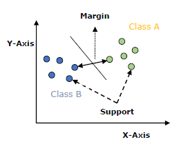
The followings are important concepts in SVM
- Improve their performance §
- At executing some task (T)
- Over time with experience (E)
The main goal of SVM is to divide the datasets into classes to find a maximum marginal hyperplane (MMH) and it can be done in the following two steps
- Improve their performance §
- At executing some task (T)
- Over time with experience (E)
Implementing SVM in Python
- Improve their performance §
- At executing some task (T)
- Over time with experience (E)
SVM Kernels
In practice, SVM algorithm is implemented with kernel that transforms an input data space into the required form. SVM uses a technique called the kernel trick in which kernel takes a low dimensional input space and transforms it into a higher dimensional space. In simple words, kernel converts non-separable problems into separable problems by adding more dimensions to it. It makes SVM more powerful, flexible and accurate. The following are some of the types of kernels used by SVM.
Linear Kernel
It can be used as a dot product between any two observations. The formula of linear kernel is as below
K(x,xi)=sum(x∗xi)
From the above formula, we can see that the product between two vectors say ð‘¥ & ð‘¥ð‘– is the sum of the multiplication of each pair of input values.
Polynomial Kernel
It is more generalized form of linear kernel and distinguish curved or nonlinear input space. Following is the formula for polynomial kernel
k(X,Xi)=1+sum(X∗Xi)^d
Here d is the degree of polynomial, which we need to specify manually in the learning algorithm.
Radial Basis Function (RBF) Kernel
RBF kernel, mostly used in SVM classification, maps input space in indefinite dimensional space. Following formula explains it mathematically
K(x,xi)=exp(−gamma∗sum(x−xi^2))
Here, gamma ranges from 0 to 1. We need to manually specify it in the learning algorithm. A good default value of gamma is 0.1.
As we implemented SVM for linearly separable data, we can implement it in Python for the data that is not linearly separable. It can be done by using kernels.
Example
The following is an example for creating an SVM classifier by using kernels. We will be using iris dataset from scikit-learn −
We will start by importing following packages
import pandas as pd
import numpy as np
from sklearn import svm, datasets
import matplotlib.pyplot as plt
Now, we need to load the input data
iris = datasets.load_iris()
From this dataset, we are taking first two features as follows
X = iris.data[:, :2]
y = iris.target
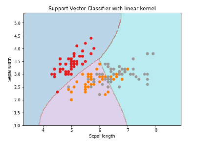
Next, we will plot the SVM boundaries with original data as follows
x_min, x_max = X[:, 0].min() - 1, X[:, 0].max() + 1
y_min, y_max = X[:, 1].min() - 1, X[:, 1].max() + 1
h = (x_max / x_min)/100
xx, yy = np.meshgrid(np.arange(x_min, x_max, h), np.arange(y_min, y_max, h))
X_plot = np.c_[xx.ravel(), yy.ravel()]
Now, we need to provide the value of regularization parameter as follows
C = 1.0
Next, SVM classifier object can be created as follows
Svc_classifier = svm.SVC(kernel='linear', C=C).fit(X, y)
Z = svc_classifier.predict(X_plot)
Z = Z.reshape(xx.shape)
plt.figure(figsize=(15, 5))
plt.subplot(121)
plt.contourf(xx, yy, Z, cmap=plt.cm.tab10, alpha=0.3)
plt.scatter(X[:, 0], X[:, 1], c=y, cmap=plt.cm.Set1)
plt.xlabel('Sepal length')
plt.ylabel('Sepal width')
plt.xlim(xx.min(), xx.max())
plt.title('Support Vector Classifier with linear kernel')
Output
Text(0.5, 1.0, 'Support Vector Classifier with linear kernel')
For creating SVM classifier with rbf kernel, we can change the kernel to rbf as follows
Svc_classifier = svm.SVC(kernel = 'rbf', gamma =‘auto’,C = C).fit(X, y)
Z = svc_classifier.predict(X_plot)
Z = Z.reshape(xx.shape)
plt.figure(figsize=(15, 5))
plt.subplot(121)
plt.contourf(xx, yy, Z, cmap = plt.cm.tab10, alpha = 0.3)
plt.scatter(X[:, 0], X[:, 1], c = y, cmap = plt.cm.Set1)
plt.xlabel('Sepal length')
plt.ylabel('Sepal width')
plt.xlim(xx.min(), xx.max())
plt.title('Support Vector Classifier with rbf kernel')
Output
Text(0.5, 1.0, 'Support Vector Classifier with rbf kernel')
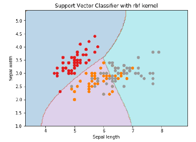
We put the value of gamma to ‘auto’ but you can provide its value between 0 to 1 also.
Pros and Cons of SVM Classifiers
Pros of SVM classifiers
SVM classifiers offers great accuracy and work well with high dimensional space. SVM classifiers basically use a subset of training points hence in result uses very less memory.
Cons of SVM classifiers
They have high training time hence in practice not suitable for large datasets. Another disadvantage is that SVM classifiers do not work well with overlapping classes.
Classification Algorithms - Decision Tree
Introduction to Decision Tree
In general, Decision tree analysis is a predictive modelling tool that can be applied across many areas. Decision trees can be constructed by an algorithmic approach that can split the dataset in different ways based on different conditions. Decisions tress are the most powerful algorithms that falls under the category of supervised algorithms.
They can be used for both classification and regression tasks. The two main entities of a tree are decision nodes, where the data is split and leaves, where we got outcome. The example of a binary tree for predicting whether a person is fit or unfit providing various information like age, eating habits and exercise habits, is given below −
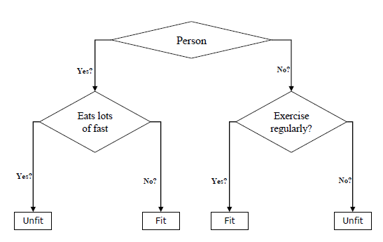
In the above decision tree, the question are decision nodes and final outcomes are leaves. We have the following two types of decision trees.
- Improve their performance §
- At executing some task (T)
- Over time with experience (E)
Implementing Decision Tree Algorithm
Gini Index
It is the name of the cost function that is used to evaluate the binary splits in the dataset and works with the categorial target variable “Success” or “Failure”.
Higher the value of Gini index, higher the homogeneity. A perfect Gini index value is 0 and worst is 0.5 (for 2 class problem). Gini index for a split can be calculated with the help of following steps −
- Improve their performance §
- At executing some task (T)
- Over time with experience (E)
Classification and Regression Tree (CART) algorithm uses Gini method to generate binary splits.
Split Creation
A split is basically including an attribute in the dataset and a value. We can create a split in dataset with the help of following three parts −
- Improve their performance §
- At executing some task (T)
- Over time with experience (E)
Building a Tree
As we know that a tree has root node and terminal nodes. After creating the root node, we can build the tree by following two parts
Part 1: Terminal node creation
While creating terminal nodes of decision tree, one important point is to decide when to stop growing tree or creating further terminal nodes. It can be done by using two criteria namely maximum tree depth and minimum node records as follows −
- Improve their performance §
- At executing some task (T)
- Over time with experience (E)
Terminal node is used to make a final prediction.
Part 2: Recursive Splitting
As we understood about when to create terminal nodes, now we can start building our tree. Recursive splitting is a method to build the tree. In this method, once a node is created, we can create the child nodes (nodes added to an existing node) recursively on each group of data, generated by splitting the dataset, by calling the same function again and again.
Prediction
After building a decision tree, we need to make a prediction about it. Basically, prediction involves navigating the decision tree with the specifically provided row of data.
We can make a prediction with the help of recursive function, as did above. The same prediction routine is called again with the left or the child right nodes.
Assumptions
The following are some of the assumptions we make while creating decision tree −
- Improve their performance §
- At executing some task (T)
- Over time with experience (E)
Implementation in Python
Example
In the following example, we are going to implement Decision Tree classifier on Pima Indian Diabetes
First, start with importing necessary python packages
import pandas as pd
from sklearn.tree import DecisionTreeClassifier
from sklearn.model_selection import train_test_split
Next, download the iris dataset from its weblink as follows
col_names = ['pregnant', 'glucose', 'bp', 'skin', 'insulin', 'bmi', 'pedigree', 'age', 'label']
pima = pd.read_csv(r"C:\pima-indians-diabetes.csv", header = None, names = col_names)
pima.head()

Now, split the dataset into features and target variable as follows
feature_cols = ['pregnant', 'insulin', 'bmi', 'age','glucose','bp','pedigree']
X = pima[feature_cols] # Features
y = pima.label # Target variable
Next, we will divide the data into train and test split. The following code will split the dataset into 70% training data and 30% of testing data
X_train, X_test, y_train, y_test = train_test_split(X, y, test_size = 0.3, random_state = 1)
Next, train the model with the help of DecisionTreeClassifier class of sklearn as follows
clf = DecisionTreeClassifier()
clf = clf.fit(X_train,y_train)
At last we need to make prediction. It can be done with the help of following script
y_pred = clf.predict(X_test)
Next, we can get the accuracy score, confusion matrix and classification report as follows
from sklearn.metrics import classification_report, confusion_matrix, accuracy_score
result = confusion_matrix(y_test, y_pred)
print("Confusion Matrix:")
print(result)
result1 = classification_report(y_test, y_pred)
print("Classification Report:",)
print (result1)
result2 = accuracy_score(y_test,y_pred)
print("Accuracy:",result2)
Output
Confusion Matrix:
  [[116 30]
  [ 46 39]]
Classification Report:
             precision    recall     f1-score    support
       0         0.72      0.79         0.75        146
       1         0.57      0.46         0.51         85
micro avg         0.67      0.67         0.67        231
macro avg         0.64      0.63         0.63        231
weighted avg      0.66      0.67         0.66        231

Accuracy: 0.670995670995671
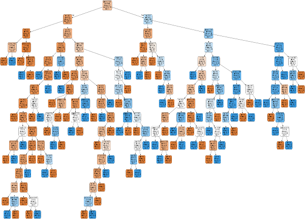
Visualizing Decision Tree
The above decision tree can be visualized with the help of following code
from sklearn.tree import export_graphviz
from sklearn.externals.six import StringIO
from IPython.display import Image
import pydotplus
dot_data = StringIO()
export_graphviz(clf, out_file=dot_data, filled=True, rounded=True,
  special_characters=True,feature_names = feature_cols,class_names=['0','1'])

graph = pydotplus.graph_from_dot_data(dot_data.getvalue())
graph.write_png('Pima_diabetes_Tree.png')
Image(graph.create_png())
Classification Algorithms - Naïve Bayes
Introduction to Naïve Bayes Algorithm
Naïve Bayes algorithms is a classification technique based on applying Bayes’ theorem with a strong assumption that all the predictors are independent to each other. In simple words, the assumption is that the presence of a feature in a class is independent to the presence of any other feature in the same class. For example, a phone may be considered as smart if it is having touch screen, internet facility, good camera etc. Though all these features are dependent on each other, they contribute independently to the probability of that the phone is a smart phone.
In Bayesian classification, the main interest is to find the posterior probabilities i.e. the probability of a label given some observed features, 𝑃(𝐿 | 𝑓𝑒𝑎𝑡𝑢𝑟𝑒𝑠). With the help of Bayes theorem, we can express this in quantitative form as follows

Here, (𝐿 | 𝑓𝑒𝑎𝑡𝑢𝑟𝑒𝑠) is the posterior probability of class.
𝑃(𝐿) is the prior probability of class.
𝑃(𝑓𝑒𝑎𝑡𝑢𝑟𝑒𝑠|𝐿) is the likelihood which is the probability of predictor given class.
𝑃(𝑓𝑒𝑎𝑡𝑢𝑟𝑒𝑠) is the prior probability of predictor.
Building model using Naïve Bayes in Python
Python library, Scikit learn is the most useful library that helps us to build a Naïve Bayes model in Python. We have the following three types of Naïve Bayes model under Scikit learn Python library
Gaussian Naïve Bayes
It is the simplest Naïve Bayes classifier having the assumption that the data from each label is drawn from a simple Gaussian distribution.
Multinomial Naïve Bayes
Another useful Naïve Bayes classifier is Multinomial Naïve Bayes in which the features are assumed to be drawn from a simple Multinomial distribution. Such kind of Naïve Bayes are most appropriate for the features that represents discrete counts.
Bernoulli Naïve Bayes
Another important model is Bernoulli Naïve Bayes in which features are assumed to be binary (0s and 1s). Text classification with ‘bag of words’ model can be an application of Bernoulli Naïve Bayes.
Example
Depending on our data set, we can choose any of the Naïve Bayes model explained above. Here, we are implementing Gaussian Naïve Bayes model in Python
We will start with required imports as follows
import numpy as np
import matplotlib.pyplot as plt
import seaborn as sns; sns.set()
Now, by using make_blobs() function of Scikit learn, we can generate blobs of points with Gaussian distribution as follows
from sklearn.datasets import make_blobs
X, y = make_blobs(300, 2, centers = 2, random_state = 2, cluster_std = 1.5)
plt.scatter(X[:, 0], X[:, 1], c = y, s = 50, cmap = 'summer');
Next, for using GaussianNB model, we need to import and make its object as follows
from sklearn.naive_bayes import GaussianNB
model_GBN = GaussianNB()
model_GNB.fit(X, y);
Now, we have to do prediction. It can be done after generating some new data as follows
rng = np.random.RandomState(0)
Xnew = [-6, -14] + [14, 18] * rng.rand(2000, 2)
ynew = model_GNB.predict(Xnew)
Next, we are plotting new data to find its boundaries
plt.scatter(X[:, 0], X[:, 1], c = y, s = 50, cmap = 'summer')
lim = plt.axis()
plt.scatter(Xnew[:, 0], Xnew[:, 1], c = ynew, s = 20, cmap = 'summer', alpha = 0.1)
plt.axis(lim);
Now, with the help of following line of codes, we can find the posterior probabilities of first and second label
yprob = model_GNB.predict_proba(Xnew)
yprob[-10:].round(3)
Output
array([[0.998, 0.002],
  [1. , 0. ],
  [0.987, 0.013],
  [1. , 0. ],
  [1. , 0. ],
  [1. , 0. ],
  [1. , 0. ],
  [1. , 0. ],
  [0. , 1. ],
  [0.986, 0.014]])
Pros & Cons
Pros
The followings are some pros of using Naïve Bayes classifiers −
- Improve their performance §
- At executing some task (T)
- Over time with experience (E)
Cons
The followings are some cons of using Naïve Bayes classifiers −
- Improve their performance §
- At executing some task (T)
- Over time with experience (E)
Applications of Naïve Bayes classification
The following are some common applications of Naïve Bayes classification
- Improve their performance §
- At executing some task (T)
- Over time with experience (E)
Classification Algorithms - Random Forest
Introduction
Random forest is a supervised learning algorithm which is used for both classification as well as regression. But however, it is mainly used for classification problems. As we know that a forest is made up of trees and more trees means more robust forest. Similarly, random forest algorithm creates decision trees on data samples and then gets the prediction from each of them and finally selects the best solution by means of voting. It is an ensemble method which is better than a single decision tree because it reduces the over-fitting by averaging the result.
Working of Random Forest Algorithm
We can understand the working of Random Forest algorithm with the help of following steps −
- Improve their performance §
- At executing some task (T)
- Over time with experience (E)
The following diagram will illustrate its working
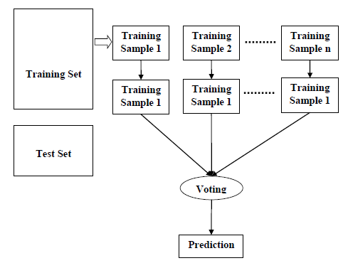
Implementation in Python
First, start with importing necessary Python packages
import numpy as np
import matplotlib.pyplot as plt
import pandas as pd
Next, download the iris dataset from its weblink as follows
path = "https://archive.ics.uci.edu/ml/machine-learning-databases/iris/iris.data"
Next, we need to assign column names to the dataset as follows
headernames = ['sepal-length', 'sepal-width', 'petal-length', 'petal-width', 'Class']
Now, we need to read dataset to pandas dataframe as follows
dataset = pd.read_csv(path, names = headernames)
dataset.head()
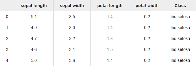
Data Preprocessing will be done with the help of following script lines.
X = dataset.iloc[:, :-1].values
y = dataset.iloc[:, 4].values
Next, we will divide the data into train and test split. The following code will split the dataset into 70% training data and 30% of testing data
from sklearn.model_selection import train_test_split
X_train, X_test, y_train, y_test = train_test_split(X, y, test_size = 0.30)
Next, train the model with the help of RandomForestClassifier class of sklearn as follows
from sklearn.ensemble import RandomForestClassifier
classifier = RandomForestClassifier(n_estimators = 50)
classifier.fit(X_train, y_train)
At last, we need to make prediction. It can be done with the help of following script
y_pred = classifier.predict(X_test)
Next, print the results as follows
from sklearn.metrics import classification_report, confusion_matrix, accuracy_score
result = confusion_matrix(y_test, y_pred)
print("Confusion Matrix:")
print(result)
result1 = classification_report(y_test, y_pred)
print("Classification Report:",)
print (result1)
result2 = accuracy_score(y_test,y_pred)
print("Accuracy:",result2)
Output
Confusion Matrix:
[[14 0 0]
  [ 0 18 1]
  [ 0 0 12]]
Classification Report:
             precision  recall  f1-score  support
   Iris-setosa   1.00    1.00      1.00       14
Iris-versicolor   1.00    0.95      0.97       19
 Iris-virginica   0.92    1.00      0.96       12

     micro avg   0.98    0.98       0.98      45
     macro avg   0.97    0.98       0.98      45
  weighted avg   0.98    0.98       0.98      45

Accuracy: 0.9777777777777777
Pros and Cons of Random Forest
Pros
The following are the advantages of Random Forest algorithm −
- Improve their performance §
- At executing some task (T)
- Over time with experience (E)
Cons
The following are the disadvantages of Random Forest algorithm −
- Improve their performance §
- At executing some task (T)
- Over time with experience (E)
Regression Algorithms - Overview
Introduction to Regression
Regression is another important and broadly used statistical and machine learning tool. The key objective of regression-based tasks is to predict output labels or responses which are continues numeric values, for the given input data. The output will be based on what the model has learned in training phase. Basically, regression models use the input data features (independent variables) and their corresponding continuous numeric output values (dependent or outcome variables) to learn specific association between inputs and corresponding outputs.
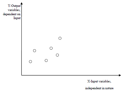
Types of Regression Models
Regression models are of following two types
Simple regression model − This is the most basic regression model in which predictions are formed from a single, univariate feature of the data.
Multiple regression model − As name implies, in this regression model the predictions are formed from multiple features of the data.
Building a Regressor in Python
Regressor model in Python can be constructed just like we constructed the classifier. Scikit-learn, a Python library for machine learning can also be used to build a regressor in Python.
In the following example, we will be building basic regression model that will fit a line to the data i.e. linear regressor. The necessary steps for building a regressor in Python are as follows −
Step 1: Importing necessary python package
For building a regressor using scikit-learn, we need to import it along with other necessary packages. We can import the by using following script
import numpy as np
from sklearn import linear_model
import sklearn.metrics as sm
import matplotlib.pyplot as plt
Step 2: Importing dataset
After importing necessary package, we need a dataset to build regression prediction model. We can import it from sklearn dataset or can use other one as per our requirement. We are going to use our saved input data. We can import it with the help of following script
input = r'C:\linear.txt'
Next, we need to load this data. We are using np.loadtxt function to load it.
input_data = np.loadtxt(input, delimiter=',')
X, y = input_data[:, :-1], input_data[:, -1]
Step 3: Organizing data into training & testing sets
As we need to test our model on unseen data hence, we will divide our dataset into two parts: a training set and a test set. The following command will perform it
training_samples = int(0.6 * len(X))
testing_samples = len(X) - num_training
X_train, y_train = X[:training_samples], y[:training_samples]
X_test, y_test = X[training_samples:], y[training_samples:]
Step 4: Model evaluation & prediction
After dividing the data into training and testing we need to build the model. We will be using LineaRegression() function of Scikit-learn for this purpose. Following command will create a linear regressor object.
reg_linear = linear_model.LinearRegression()
Next, train this model with the training samples as follows
reg_linear.fit(X_train, y_train)
Now, at last we need to do the prediction with the testing data.
y_test_pred = reg_linear.predict(X_test)
Step 5: Plot & visualization
After prediction, we can plot and visualize it with the help of following script
plt.scatter(X_test, y_test, color = 'red')
plt.plot(X_test, y_test_pred, color = 'black', linewidth = 2)
plt.xticks(())
plt.yticks(())
plt.show()
Output
In the above output, we can see the regression line between the data points.
Step 6: Performance computation − We can also compute the performance of our regression model with the help of various performance metrics as follows.
print("Regressor model performance:")
print("Mean absolute error(MAE) =", round(sm.mean_absolute_error(y_test, y_test_pred), 2))
print("Mean squared error(MSE) =", round(sm.mean_squared_error(y_test, y_test_pred), 2))
print("Median absolute error =", round(sm.median_absolute_error(y_test, y_test_pred), 2))
print("Explain variance score =", round(sm.explained_variance_score(y_test, y_test_pred), 2))
print("R2 score =", round(sm.r2_score(y_test, y_test_pred), 2))
Output
Regressor model performance:
Mean absolute error(MAE) = 1.78
Mean squared error(MSE) = 3.89
Median absolute error = 2.01
Explain variance score = -0.09
R2 score = -0.09
Types of ML Regression Algorithms
The most useful and popular ML regression algorithm is Linear regression algorithm which further divided into two types namely −
- Improve their performance §
- At executing some task (T)
- Over time with experience (E)
We will discuss about it and implement it in Python in the next chapter.
Applications
The applications of ML regression algorithms are as follows −
Forecasting or Predictive analysis − One of the important uses of regression is forecasting or predictive analysis. For example, we can forecast GDP, oil prices or in simple words the quantitative data that changes with the passage of time.
Optimization − We can optimize business processes with the help of regression. For example, a store manager can create a statistical model to understand the peek time of coming of customers.
Error correction − In business, taking correct decision is equally important as optimizing the business process. Regression can help us to take correct decision as well in correcting the already implemented decision.
Economics − It is the most used tool in economics. We can use regression to predict supply, demand, consumption, inventory investment etc.
Finance − A financial company is always interested in minimizing the risk portfolio and want to know the factors that affects the customers. All these can be predicted with the help of regression model.
Regression Algorithms - Linear Regression
Introduction to Linear Regression
Linear regression may be defined as the statistical model that analyzes the linear relationship between a dependent variable with given set of independent variables. Linear relationship between variables means that when the value of one or more independent variables will change (increase or decrease), the value of dependent variable will also change accordingly (increase or decrease).
Mathematically the relationship can be represented with the help of following equation
Y=mX+b
Here, Y is the dependent variable we are trying to predict.
X is the dependent variable we are using to make predictions.
m is the slop of the regression line which represents the effect X has on Y
b is a constant, known as the 𝑌Y-intercept. If X = 0,Y would be equal to 𝑏b.
Furthermore, the linear relationship can be positive or negative in nature as explained below −
Positive Linear Relationship
A linear relationship will be called positive if both independent and dependent variable increases. It can be understood with the help of following graph
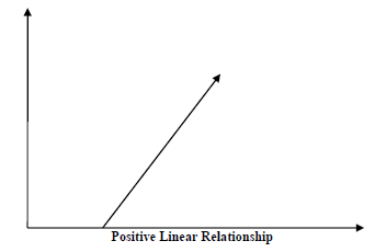
Negative Linear relationship
A linear relationship will be called positive if independent increases and dependent variable decreases. It can be understood with the help of following graph
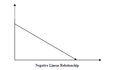
Types of Linear Regression
Linear regression is of the following two types
- Improve their performance §
- At executing some task (T)
- Over time with experience (E)
Assumptions
The following are some assumptions about dataset that is made by Linear Regression model −
Multi-collinearity − Linear regression model assumes that there is very little or no multi-collinearity in the data. Basically, multi-collinearity occurs when the independent variables or features have dependency in them.
Auto-correlation − Another assumption Linear regression model assumes is that there is very little or no auto-correlation in the data. Basically, auto-correlation occurs when there is dependency between residual errors.
Relationship between variables − Linear regression model assumes that the relationship between response and feature variables must be linear.
Clustering Algorithms - Overview
Introduction to Clustering
Clustering methods are one of the most useful unsupervised ML methods. These methods are used to find similarity as well as the relationship patterns among data samples and then cluster those samples into groups having similarity based on features.
Clustering is important because it determines the intrinsic grouping among the present unlabeled data. They basically make some assumptions about data points to constitute their similarity. Each assumption will construct different but equally valid clusters.
For example, below is the diagram which shows clustering system grouped together the similar kind of data in different clusters
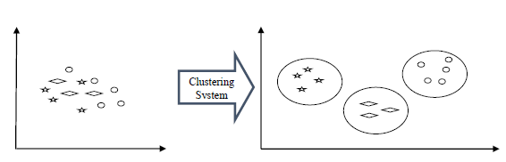
Cluster Formation Methods
It is not necessary that clusters will be formed in spherical form. Followings are some other cluster formation methods −
Density-based
In these methods, the clusters are formed as the dense region. The advantage of these methods is that they have good accuracy as well as good ability to merge two clusters. Ex. Density-Based Spatial Clustering of Applications with Noise (DBSCAN), Ordering Points to identify Clustering structure (OPTICS) etc.
Hierarchical-based
In these methods, the clusters are formed as a tree type structure based on the hierarchy. They have two categories namely, Agglomerative (Bottom up approach) and Divisive (Top down approach). Ex. Clustering using Representatives (CURE), Balanced iterative Reducing Clustering using Hierarchies (BIRCH) etc.
Partitioning
In these methods, the clusters are formed by portioning the objects into k clusters. Number of clusters will be equal to the number of partitions. Ex. K-means, Clustering Large Applications based upon randomized Search (CLARANS).
Grid
In these methods, the clusters are formed as a grid like structure. The advantage of these methods is that all the clustering operation done on these grids are fast and independent of the number of data objects. Ex. Statistical Information Grid (STING), Clustering in Quest (CLIQUE).
Measuring Clustering Performance
One of the most important consideration regarding ML model is assessing its performance or you can say model’s quality. In case of supervised learning algorithms, assessing the quality of our model is easy because we already have labels for every example.
On the other hand, in case of unsupervised learning algorithms we are not that much blessed because we deal with unlabeled data. But still we have some metrics that give the practitioner an insight about the happening of change in clusters depending on algorithm.
Before we deep dive into such metrics, we must understand that these metrics only evaluates the comparative performance of models against each other rather than measuring the validity of the model’s prediction. Followings are some of the metrics that we can deploy on clustering algorithms to measure the quality of model −
Silhouette Analysis
Silhouette analysis used to check the quality of clustering model by measuring the distance between the clusters. It basically provides us a way to assess the parameters like number of clusters with the help of Silhouette score. This score measures how close each point in one cluster is to points in the neighboring clusters.
Analysis of Silhouette Score
- Improve their performance §
- At executing some task (T)
- Over time with experience (E)
Types of ML Clustering Algorithms
The following are the most important and useful ML clustering algorithms
K-means Clustering
This clustering algorithm computes the centroids and iterates until we it finds optimal centroid. It assumes that the number of clusters are already known. It is also called flat clustering algorithm. The number of clusters identified from data by algorithm is represented by ‘K’ in K-means.
Mean-Shift Algorithm
It is another powerful clustering algorithm used in unsupervised learning. Unlike K-means clustering, it does not make any assumptions hence it is a non-parametric algorithm.
Hierarchical Clustering
It is another unsupervised learning algorithm that is used to group together the unlabeled data points having similar characteristics.
We will be discussing all these algorithms in detail in the upcoming chapters.
Applications of Clustering
We can find clustering useful in the following areas −
Data summarization and compression − Clustering is widely used in the areas where we require data summarization, compression and reduction as well. The examples are image processing and vector quantization.
Collaborative systems and customer segmentation − Since clustering can be used to find similar products or same kind of users, it can be used in the area of collaborative systems and customer segmentation.
Serve as a key intermediate step for other data mining tasks − Cluster analysis can generate a compact summary of data for classification, testing, hypothesis generation; hence, it serves as a key intermediate step for other data mining tasks also.
Trend detection in dynamic data − Clustering can also be used for trend detection in dynamic data by making various clusters of similar trends.
Social network analysis − Clustering can be used in social network analysis. The examples are generating sequences in images, videos or audios.
Biological data analysis − Clustering can also be used to make clusters of images, videos hence it can successfully be used in biological data analysis.
ML - Clustering K-Means Algorithm
Introduction to K-Means Algorithm
K-means clustering algorithm computes the centroids and iterates until we it finds optimal centroid. It assumes that the number of clusters are already known. It is also called flat clustering algorithm. The number of clusters identified from data by algorithm is represented by ‘K’ in K-means.
In this algorithm, the data points are assigned to a cluster in such a manner that the sum of the squared distance between the data points and centroid would be minimum. It is to be understood that less variation within the clusters will lead to more similar data points within same cluster.
Working of K-Means Algorithm
We can understand the working of K-Means clustering algorithm with the help of following steps
Step 1 − First, we need to specify the number of clusters, K, need to be generated by this algorithm.
Step 2 − Next, randomly select K data points and assign each data point to a cluster. In simple words, classify the data based on the number of data points.
Step 3 − Now it will compute the cluster centroids.
Step 4 − Next, keep iterating the following until we find optimal centroid which is the assignment of data points to the clusters that are not changing any more
- Improve their performance §
- At executing some task (T)
- Over time with experience (E)
K-means follows Expectation-Maximization approach to solve the problem. The Expectation-step is used for assigning the data points to the closest cluster and the Maximization-step is used for computing the centroid of each cluster.
While working with K-means algorithm we need to take care of the following things −
- Improve their performance §
- At executing some task (T)
- Over time with experience (E)
Implementation in Python
The following two examples of implementing K-Means clustering algorithm will help us in its better understanding
Example 1
It is a simple example to understand how k-means works. In this example, we are going to first generate 2D dataset containing 4 different blobs and after that will apply k-means algorithm to see the result.
First, we will start by importing the necessary packages
%matplotlib inline
import matplotlib.pyplot as plt
import seaborn as sns; sns.set()
import numpy as np
from sklearn.cluster import KMeans
The following code will generate the 2D, containing four blobs
from sklearn.datasets.samples_generator import make_blobs
X, y_true = make_blobs(n_samples = 400, centers = 4, cluster_std = 0.60, random_state = 0)
Next, the following code will help us to visualize the dataset
plt.scatter(X[:, 0], X[:, 1], s = 20);
plt.show()
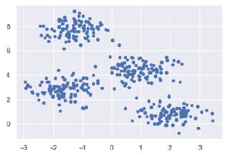
Next, make an object of KMeans along with providing number of clusters, train the model and do the prediction as follows
kmeans = KMeans(n_clusters = 4)
kmeans.fit(X)
y_kmeans = kmeans.predict(X)
Now, with the help of following code we can plot and visualize the cluster’s centers picked by k-means Python estimator
from sklearn.datasets.samples_generator import make_blobs
X, y_true = make_blobs(n_samples = 400, centers = 4, cluster_std = 0.60, random_state = 0)
Next, the following code will help us to visualize the dataset
plt.scatter(X[:, 0], X[:, 1], c = y_kmeans, s = 20, cmap = 'summer')
centers = kmeans.cluster_centers_
plt.scatter(centers[:, 0], centers[:, 1], c = 'blue', s = 100, alpha = 0.9);
plt.show()
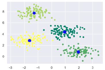
Example 2
Let us move to another example in which we are going to apply K-means clustering on simple digits dataset. K-means will try to identify similar digits without using the original label information.
First, we will start by importing the necessary packages
%matplotlib inline
import matplotlib.pyplot as plt
import seaborn as sns; sns.set()
import numpy as np
from sklearn.cluster import KMeans
Next, load the digit dataset from sklearn and make an object of it. We can also find number of rows and columns in this dataset as follows
from sklearn.datasets import load_digits
digits = load_digits()
digits.data.shape
Output
(1797, 64)
The above output shows that this dataset is having 1797 samples with 64 features.
We can perform the clustering as we did in Example 1 above
kmeans = KMeans(n_clusters = 10, random_state = 0)
clusters = kmeans.fit_predict(digits.data)
kmeans.cluster_centers_.shape
Output
(10, 64)
The above output shows that K-means created 10 clusters with 64 features.
fig, ax = plt.subplots(2, 5, figsize=(8, 3))
centers = kmeans.cluster_centers_.reshape(10, 8, 8)
for axi, center in zip(ax.flat, centers):
axi.set(xticks=[], yticks=[])
axi.imshow(center, interpolation='nearest', cmap=plt.cm.binary)
Output
As output, we will get following image showing clusters centers learned by k-means.
The following lines of code will match the learned cluster labels with the true labels found in them
from scipy.stats import mode
labels = np.zeros_like(clusters)
for i in range(10):
  mask = (clusters == i)
  labels[mask] = mode(digits.target[mask])[0]
Next, we can check the accuracy as follows
from sklearn.metrics import accuracy_score
accuracy_score(digits.target, labels)
Output
0.7935447968836951
The above output shows that the accuracy is around 80%.
Advantages and Disadvantages
Advantages
The following are some advantages of K-Means clustering algorithms −
- Improve their performance §
- At executing some task (T)
- Over time with experience (E)
Disadvantages
The following are some disadvantages of K-Means clustering algorithms −
- Improve their performance §
- At executing some task (T)
- Over time with experience (E)
Applications of K-Means Clustering Algorithm
The main goals of cluster analysis are
- Improve their performance §
- At executing some task (T)
- Over time with experience (E)
To fulfill the above-mentioned goals, K-means clustering is performing well enough. It can be used in following applications −
- Improve their performance §
- At executing some task (T)
- Over time with experience (E)
ML - Clustering Mean Shift Algorithm
Introduction to Mean-Shift Algorithm
As discussed earlier, it is another powerful clustering algorithm used in unsupervised learning. Unlike K-means clustering, it does not make any assumptions; hence it is a non-parametric algorithm.
Mean-shift algorithm basically assigns the datapoints to the clusters iteratively by shifting points towards the highest density of datapoints i.e. cluster centroid.
The difference between K-Means algorithm and Mean-Shift is that later one does not need to specify the number of clusters in advance because the number of clusters will be determined by the algorithm w.r.t data.
Working of Mean-Shift Algorithm
We can understand the working of Mean-Shift clustering algorithm with the help of following steps −
- Improve their performance §
- At executing some task (T)
- Over time with experience (E)
Implementation in Python
It is a simple example to understand how Mean-Shift algorithm works. In this example, we are going to first generate 2D dataset containing 4 different blobs and after that will apply Mean-Shift algorithm to see the result.
%matplotlib inline
import numpy as np
from sklearn.cluster import MeanShift
import matplotlib.pyplot as plt
from matplotlib import style
style.use("ggplot")
from sklearn.datasets.samples_generator import make_blobs
centers = [[3,3,3],[4,5,5],[3,10,10]]
X, _ = make_blobs(n_samples = 700, centers = centers, cluster_std = 0.5)
plt.scatter(X[:,0],X[:,1])
plt.show()
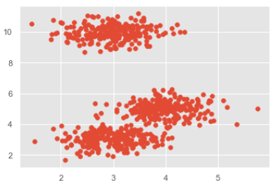
ms = MeanShift()
ms.fit(X)
labels = ms.labels_
cluster_centers = ms.cluster_centers_
print(cluster_centers)
n_clusters_ = len(np.unique(labels))
print("Estimated clusters:", n_clusters_)
colors = 10*['r.','g.','b.','c.','k.','y.','m.']

for i in range(len(X)):
  plt.plot(X[i][0], X[i][1], colors[labels[i]], markersize = 3)
plt.scatter(cluster_centers[:,0],cluster_centers[:,1],
  marker = ".",color = 'k', s = 20, linewidths = 5, zorder = 10)
plt.show()
Output
[[ 2.98462798 9.9733794 10.02629344]
[ 3.94758484 4.99122771 4.99349433]
[ 3.00788996 3.03851268 2.99183033]]
Estimated clusters: 3
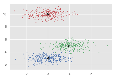
Advantages and Disadvantages
Advantages
The following are some advantages of Mean-Shift clustering algorithm −
- Improve their performance §
- At executing some task (T)
- Over time with experience (E)
Disadvantages
The following are some disadvantages of Mean-Shift clustering algorithm
- Improve their performance §
- At executing some task (T)
- Over time with experience (E)
Machine Learning - Hierarchical Clustering
Introduction to Hierarchical Clustering
Hierarchical clustering is another unsupervised learning algorithm that is used to group together the unlabeled data points having similar characteristics. Hierarchical clustering algorithms falls into following two categories.
Agglomerative hierarchical algorithms − In agglomerative hierarchical algorithms, each data point is treated as a single cluster and then successively merge or agglomerate (bottom-up approach) the pairs of clusters. The hierarchy of the clusters is represented as a dendrogram or tree structure.
Divisive hierarchical algorithms − On the other hand, in divisive hierarchical algorithms, all the data points are treated as one big cluster and the process of clustering involves dividing (Top-down approach) the one big cluster into various small clusters.
Steps to Perform Agglomerative Hierarchical Clustering
We are going to explain the most used and important Hierarchical clustering i.e. agglomerative. The steps to perform the same is as follows −
- Improve their performance §
- At executing some task (T)
- Over time with experience (E)
Role of Dendrograms in Agglomerative Hierarchical Clustering
As we discussed in the last step, the role of dendrogram starts once the big cluster is formed. Dendrogram will be used to split the clusters into multiple cluster of related data points depending upon our problem. It can be understood with the help of following example
Example 1
To understand, let us start with importing the required libraries as follows
%matplotlib inline
import matplotlib.pyplot as plt
import numpy as np
Next, we will be plotting the datapoints we have taken for this example
X = np.array(
  [[7,8],[12,20],[17,19],[26,15],[32,37],[87,75],[73,85], [62,80],[73,60],[87,96],])
labels = range(1, 11)
plt.figure(figsize = (10, 7))
plt.subplots_adjust(bottom = 0.1)
plt.scatter(X[:,0],X[:,1], label = 'True Position')
for label, x, y in zip(labels, X[:, 0], X[:, 1]):
  plt.annotate(
     label,xy = (x, y), xytext = (-3, 3),textcoords = 'offset points', ha = 'right', va = 'bottom')
plt.show()
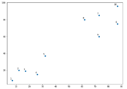
From the above diagram, it is very easy to see that we have two clusters in out datapoints but in the real world data, there can be thousands of clusters. Next, we will be plotting the dendrograms of our datapoints by using Scipy library
from scipy.cluster.hierarchy import dendrogram, linkage
from matplotlib import pyplot as plt
linked = linkage(X, 'single')
labelList = range(1, 11)
plt.figure(figsize = (10, 7))
dendrogram(linked, orientation = 'top',labels = labelList,
  distance_sort ='descending',show_leaf_counts = True)
plt.show()
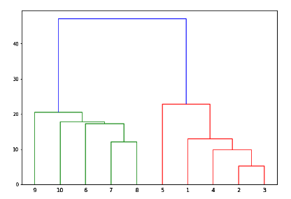
Now, once the big cluster is formed, the longest vertical distance is selected. A vertical line is then drawn through it as shown in the following diagram. As the horizontal line crosses the blue line at two points, the number of clusters would be two.
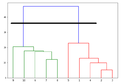
Next, we need to import the class for clustering and call its fit_predict method to predict the cluster. We are importing AgglomerativeClustering class of sklearn.cluster library
from sklearn.cluster import AgglomerativeClustering
cluster = AgglomerativeClustering(n_clusters = 2, affinity = 'euclidean', linkage = 'ward')
cluster.fit_predict(X)
Next, plot the cluster with the help of following code
plt.scatter(X[:,0],X[:,1], c = cluster.labels_, cmap = 'rainbow')
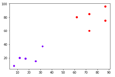
The above diagram shows the two clusters from our datapoints.
Example 2
As we understood the concept of dendrograms from the simple example discussed above, let us move to another example in which we are creating clusters of the data point in Pima Indian Diabetes Dataset by using hierarchical clustering.
import matplotlib.pyplot as plt
import pandas as pd
%matplotlib inline
import numpy as np
from pandas import read_csv
path = r"C:\pima-indians-diabetes.csv"
headernames = ['preg', 'plas', 'pres', 'skin', 'test', 'mass', 'pedi', 'age', 'class']
data = read_csv(path, names = headernames)
array = data.values
X = array[:,0:8]
Y = array[:,8]
data.shape
(768, 9)
data.head()
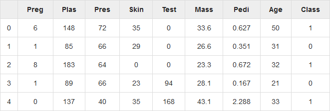
patient_data = data.iloc[:, 3:5].values
import scipy.cluster.hierarchy as shc
plt.figure(figsize = (10, 7))
plt.title("Patient Dendograms")
dend = shc.dendrogram(shc.linkage(data, method = 'ward'))
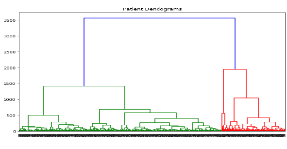
from sklearn.cluster import AgglomerativeClustering
cluster = AgglomerativeClustering(n_clusters = 4, affinity = 'euclidean', linkage = 'ward')
cluster.fit_predict(patient_data)
plt.figure(figsize = (10, 7))
plt.scatter(patient_data[:,0], patient_data[:,1], c = cluster.labels_, cmap = 'rainbow')
KNN Algorithm - Finding Nearest Neighbors
Introduction
K-nearest neighbors (KNN) algorithm is a type of supervised ML algorithm which can be used for both classification as well as regression predictive problems. However, it is mainly used for classification predictive problems in industry. The following two properties would define KNN well −
- Improve their performance §
- At executing some task (T)
- Over time with experience (E)
Working of KNN Algorithm
K-nearest neighbors (KNN) algorithm uses ‘feature similarity’ to predict the values of new datapoints which further means that the new data point will be assigned a value based on how closely it matches the points in the training set. We can understand its working with the help of following steps −
Step 1 − For implementing any algorithm, we need dataset. So during the first step of KNN, we must load the training as well as test data.
Step 2 − Next, we need to choose the value of K i.e. the nearest data points. K can be any integer.
Step 3 − For each point in the test data do the following −
- Improve their performance §
- At executing some task (T)
- Over time with experience (E)
Step 4 − End
Example
The following is an example to understand the concept of K and working of KNN algorithm
Suppose we have a dataset which can be plotted as follows
Now, we need to classify new data point with black dot (at point 60,60) into blue or red class. We are assuming K = 3 i.e. it would find three nearest data points. It is shown in the next diagram
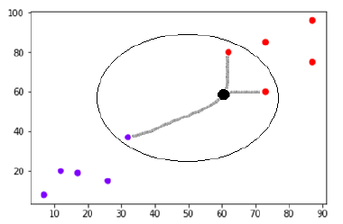
We can see in the above diagram the three nearest neighbors of the data point with black dot. Among those three, two of them lies in Red class hence the black dot will also be assigned in red class.
Implementation in Python
As we know K-nearest neighbors (KNN) algorithm can be used for both classification as well as regression. The following are the recipes in Python to use KNN as classifier as well as regressor
KNN as Classifier
First, start with importing necessary python packages
import numpy as np
import matplotlib.pyplot as plt
import pandas as pd
Next, download the iris dataset from its weblink as follows
path = "https://archive.ics.uci.edu/ml/machine-learning-databases/iris/iris.data"
Next, we need to assign column names to the dataset as follows
headernames = ['sepal-length', 'sepal-width', 'petal-length', 'petal-width', 'Class']
Now, we need to read dataset to pandas dataframe as follows −
dataset = pd.read_csv(path, names = headernames)
dataset.head()

Data Preprocessing will be done with the help of following script lines.
X = dataset.iloc[:, :-1].values
y = dataset.iloc[:, 4].values
Next, we will divide the data into train and test split. Following code will split the dataset into 60% training data and 40% of testing data
from sklearn.model_selection import train_test_split
X_train, X_test, y_train, y_test = train_test_split(X, y, test_size = 0.40)
Next, data scaling will be done as follows
from sklearn.preprocessing import StandardScaler
scaler = StandardScaler()
scaler.fit(X_train)
X_train = scaler.transform(X_train)
X_test = scaler.transform(X_test)
Next, train the model with the help of KNeighborsClassifier class of sklearn as follows
from sklearn.neighbors import KNeighborsClassifier
classifier = KNeighborsClassifier(n_neighbors = 8)
classifier.fit(X_train, y_train)
At last we need to make prediction. It can be done with the help of following script
y_pred = classifier.predict(X_test)
Next, print the results as follows
from sklearn.metrics import classification_report, confusion_matrix, accuracy_score
result = confusion_matrix(y_test, y_pred)
print("Confusion Matrix:")
print(result)
result1 = classification_report(y_test, y_pred)
print("Classification Report:",)
print (result1)
result2 = accuracy_score(y_test,y_pred)
print("Accuracy:",result2)
Output
Confusion Matrix:
[[21 0 0]
[ 0 16 0]
[ 0 7 16]]
Classification Report:
                 precision  recall  f1-score  support
   Iris-setosa       1.00    1.00      1.00       21
Iris-versicolor       0.70    1.00      0.82       16
 Iris-virginica       1.00    0.70      0.82       23
     micro avg       0.88    0.88      0.88       60
     macro avg       0.90     0.90      0.88       60
  weighted avg       0.92    0.88      0.88       60

Accuracy: 0.8833333333333333
KNN as Regressor
First, start with importing necessary Python packages
import numpy as np
import pandas as pd
Next, download the iris dataset from its weblink as follows
path = "https://archive.ics.uci.edu/ml/machine-learning-databases/iris/iris.data"
Next, we need to assign column names to the dataset as follows
headernames = ['sepal-length', 'sepal-width', 'petal-length', 'petal-width', 'Class']
Now, we need to read dataset to pandas dataframe as follows
data = pd.read_csv(url, names = headernames)
array = data.values
X = array[:,:2]
Y = array[:,2]
data.shape
output:(150, 5)
Next, import KNeighborsRegressor from sklearn to fit the model
from sklearn.neighbors import KNeighborsRegressor
knnr = KNeighborsRegressor(n_neighbors = 10)
knnr.fit(X, y)
At last, we can find the MSE as follows
print ("The MSE is:",format(np.power(y-knnr.predict(X),2).mean()))
Output
The MSE is: 0.12226666666666669
Pros and Cons of KNN
Pros
- Improve their performance §
- At executing some task (T)
- Over time with experience (E)
Cons
- Improve their performance §
- At executing some task (T)
- Over time with experience (E)
Applications of KNN
The following are some of the areas in which KNN can be applied successfully −
Banking System
KNN can be used in banking system to predict weather an individual is fit for loan approval? Does that individual have the characteristics similar to the defaulters one?
Calculating Credit Ratings
KNN algorithms can be used to find an individual’s credit rating by comparing with the persons having similar traits.
Politics
With the help of KNN algorithms, we can classify a potential voter into various classes like “Will Vote”, “Will not Vote”, “Will Vote to Party ‘Congress’, “Will Vote to Party ‘BJP’.
Other areas in which KNN algorithm can be used are Speech Recognition, Handwriting Detection, Image Recognition and Video Recognition.
Machine Learning - Performance Metrics
There are various metrics which we can use to evaluate the performance of ML algorithms, classification as well as regression algorithms. We must carefully choose the metrics for evaluating ML performance because −
- Improve their performance §
- At executing some task (T)
- Over time with experience (E)
Performance Metrics for Classification Problems
We have discussed classification and its algorithms in the previous chapters. Here, we are going to discuss various performance metrics that can be used to evaluate predictions for classification problems.
Confusion Matrix
It is the easiest way to measure the performance of a classification problem where the output can be of two or more type of classes. A confusion matrix is nothing but a table with two dimensions viz. “Actual” and “Predicted” and furthermore, both the dimensions have “True Positives (TP)”, “True Negatives (TN)”, “False Positives (FP)”, “False Negatives (FN)” as shown below
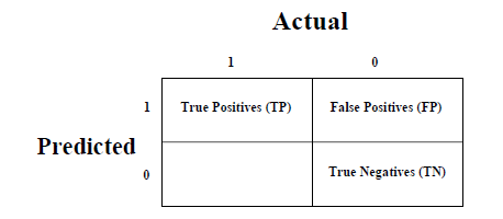
Explanation of the terms associated with confusion matrix are as follows −
- Improve their performance §
- At executing some task (T)
- Over time with experience (E)
We can use confusion_matrix function of sklearn.metrics to compute Confusion Matrix of our classification model.
Classification Accuracy
It is most common performance metric for classification algorithms. It may be defined as the number of correct predictions made as a ratio of all predictions made. We can easily calculate it by confusion matrix with the help of following formula

We can use accuracy_score function of sklearn.metrics to compute accuracy of our classification model.
Classification Report
This report consists of the scores of Precisions, Recall, F1 and Support. They are explained as follows
Precision
Precision, used in document retrievals, may be defined as the number of correct documents returned by our ML model. We can easily calculate it by confusion matrix with the help of following formula

Recall or Sensitivity
Recall may be defined as the number of positives returned by our ML model. We can easily calculate it by confusion matrix with the help of following formula.

Specificity
Specificity, in contrast to recall, may be defined as the number of negatives returned by our ML model. We can easily calculate it by confusion matrix with the help of following formula

Support
Support may be defined as the number of samples of the true response that lies in each class of target values.
F1 Score
This score will give us the harmonic mean of precision and recall. Mathematically, F1 score is the weighted average of the precision and recall. The best value of F1 would be 1 and worst would be 0. We can calculate F1 score with the help of following formula −
F1=2∗(precision∗recall)/(precision+recall)
F1 score is having equal relative contribution of precision and recall.
We can use classification_report function of sklearn.metrics to get the classification report of our classification model.
AUC (Area Under ROC curve)
AUC (Area Under Curve)-ROC (Receiver Operating Characteristic) is a performance metric, based on varying threshold values, for classification problems. As name suggests, ROC is a probability curve and AUC measure the separability. In simple words, AUC-ROC metric will tell us about the capability of model in distinguishing the classes. Higher the AUC, better the model.
Mathematically, it can be created by plotting TPR (True Positive Rate) i.e. Sensitivity or recall vs FPR (False Positive Rate) i.e. 1-Specificity, at various threshold values. Following is the graph showing ROC, AUC having TPR at y-axis and FPR at x-axis
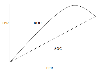
We can use roc_auc_score function of sklearn.metrics to compute AUC-ROC.
LOGLOSS (Logarithmic Loss)
It is also called Logistic regression loss or cross-entropy loss. It basically defined on probability estimates and measures the performance of a classification model where the input is a probability value between 0 and 1. It can be understood more clearly by differentiating it with accuracy. As we know that accuracy is the count of predictions (predicted value = actual value) in our model whereas Log Loss is the amount of uncertainty of our prediction based on how much it varies from the actual label. With the help of Log Loss value, we can have more accurate view of the performance of our model. We can use log_loss function of sklearn.metrics to compute Log Loss.
Example
The following is a simple recipe in Python which will give us an insight about how we can use the above explained performance metrics on binary classification model
from sklearn.metrics import confusion_matrix
from sklearn.metrics import accuracy_score
from sklearn.metrics import classification_report
from sklearn.metrics import roc_auc_score
from sklearn.metrics import log_loss
X_actual = [1, 1, 0, 1, 0, 0, 1, 0, 0, 0]
Y_predic = [1, 0, 1, 1, 1, 0, 1, 1, 0, 0]
results = confusion_matrix(X_actual, Y_predic)
print ('Confusion Matrix :')
print(results)
print ('Accuracy Score is',accuracy_score(X_actual, Y_predic))
print ('Classification Report : ')
print (classification_report(X_actual, Y_predic))
print('AUC-ROC:',roc_auc_score(X_actual, Y_predic))
print('LOGLOSS Value is',log_loss(X_actual, Y_predic))
Output
Confusion Matrix :
[[3 3]
[1 3]]
Accuracy Score is 0.6
Classification Report :
              precision  recall  f1-score  support
          0       0.75    0.50      0.60        6
          1       0.50    0.75      0.60        4
  micro avg       0.60    0.60      0.60       10
  macro avg       0.62    0.62      0.60       10
weighted avg       0.65    0.60      0.60       10
AUC-ROC: 0.625
LOGLOSS Value is 13.815750437193334
Performance Metrics for Regression Problems
We have discussed regression and its algorithms in previous chapters. Here, we are going to discuss various performance metrics that can be used to evaluate predictions for regression problems.
Mean Absolute Error (MAE)
It is the simplest error metric used in regression problems. It is basically the sum of average of the absolute difference between the predicted and actual values. In simple words, with MAE, we can get an idea of how wrong the predictions were. MAE does not indicate the direction of the model i.e. no indication about underperformance or overperformance of the model. The following is the formula to calculate MAE −

Here,y = Actual Output Values
And Y^ = Predicted Output Values.
We can use mean_absolute_error function of sklearn.metrics to compute MAE.
Mean Square Error (MSE)
MSE is like the MAE, but the only difference is that the it squares the difference of actual and predicted output values before summing them all instead of using the absolute value. The difference can be noticed in the following equation

Here,Y = Actual Output Values
And Y^= Predicted Output Values.
We can use mean_squared_error function of sklearn.metrics to compute MSE.
R Squared (R2)
R Squared metric is generally used for explanatory purpose and provides an indication of the goodness or fit of a set of predicted output values to the actual output values. The following formula will help us understanding it

In the above equation, numerator is MSE and the denominator is the variance in Y values.
We can use r2_score function of sklearn.metrics to compute R squared value.
Example
The following is a simple recipe in Python which will give us an insight about how we can use the above explained performance metrics on regression model
from sklearn.metrics import r2_score
from sklearn.metrics import mean_absolute_error
from sklearn.metrics import mean_squared_error
X_actual = [5, -1, 2, 10]
Y_predic = [3.5, -0.9, 2, 9.9]
print ('R Squared =',r2_score(X_actual, Y_predic))
print ('MAE =',mean_absolute_error(X_actual, Y_predic))
print ('MSE =',mean_squared_error(X_actual, Y_predic))
Output
R Squared = 0.9656060606060606
MAE = 0.42499999999999993
MSE = 0.5674999999999999
Machine Learning - Automatic Workflows
Introduction
In order to execute and produce results successfully, a machine learning model must automate some standard workflows. The process of automate these standard workflows can be done with the help of Scikit-learn Pipelines. From a data scientist’s perspective, pipeline is a generalized, but very important concept. It basically allows data flow from its raw format to some useful information. The working of pipelines can be understood with the help of following diagram
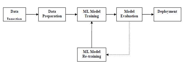
The blocks of ML pipelines are as follows
Data ingestion − As the name suggests, it is the process of importing the data for use in ML project. The data can be extracted in real time or batches from single or multiple systems. It is one of the most challenging steps because the quality of data can affect the whole ML model.
Data Preparation − After importing the data, we need to prepare data to be used for our ML model. Data preprocessing is one of the most important technique of data preparation.
ML Model Training − Next step is to train our ML model. We have various ML algorithms like supervised, unsupervised, reinforcement to extract the features from data, and make predictions.
Model Evaluation − Next, we need to evaluate the ML model. In case of AutoML pipeline, ML model can be evaluated with the help of various statistical methods and business rules.
ML Model retraining − In case of AutoML pipeline, it is not necessary that the first model is best one. The first model is considered as a baseline model and we can train it repeatably to increase model’s accuracy.
Deployment − At last, we need to deploy the model. This step involves applying and migrating the model to business operations for their use.
Challenges Accompanying ML Pipelines
In order to create ML pipelines, data scientists face many challenges. These challenges fall into the following three categories
Quality of Data
The success of any ML model depends heavily on the quality of data. If the data we are providing to ML model is not accurate, reliable and robust, then we are going to end with wrong or misleading output.
Data Reliability
Another challenge associated with ML pipelines is the reliability of data we are providing to the ML model. As we know, there can be various sources from which data scientist can acquire data but to get the best results, it must be assured that the data sources are reliable and trusted.
Data Accessibility
To get the best results out of ML pipelines, the data itself must be accessible which requires consolidation, cleansing and curation of data. As a result of data accessibility property, metadata will be updated with new tags.
Modelling ML Pipeline and Data Preparation
Data leakage, happening from training dataset to testing dataset, is an important issue for data scientist to deal with while preparing data for ML model. Generally, at the time of data preparation, data scientist uses techniques like standardization or normalization on entire dataset before learning. But these techniques cannot help us from the leakage of data because the training dataset would have been influenced by the scale of the data in the testing dataset.
By using ML pipelines, we can prevent this data leakage because pipelines ensure that data preparation like standardization is constrained to each fold of our cross-validation procedure.
Example
The following is an example in Python that demonstrate data preparation and model evaluation workflow. For this purpose, we are using Pima Indian Diabetes dataset from Sklearn. First, we will be creating pipeline that standardized the data. Then a Linear Discriminative analysis model will be created and at last the pipeline will be evaluated using 10-fold cross validation.
First, import the required packages as follows
from pandas import read_csv
from sklearn.model_selection import KFold
from sklearn.model_selection import cross_val_score
from sklearn.preprocessing import StandardScaler
from sklearn.pipeline import Pipeline
from sklearn.discriminant_analysis import LinearDiscriminantAnalysis
Now, we need to load the Pima diabetes dataset as did in previous examples
path = r"C:\pima-indians-diabetes.csv"
headernames = ['preg', 'plas', 'pres', 'skin', 'test', 'mass', 'pedi', 'age', 'class']
data = read_csv(path, names = headernames)
array = data.values
Next, we will create a pipeline with the help of the following code
estimators = []
estimators.append(('standardize', StandardScaler()))
estimators.append(('lda', LinearDiscriminantAnalysis()))
model = Pipeline(estimators)
At last, we are going to evaluate this pipeline and output its accuracy as follows
kfold = KFold(n_splits = 20, random_state = 7)
results = cross_val_score(model, X, Y, cv = kfold)
print(results.mean())
Output
0.7790148448043184
The above output is the summary of accuracy of the setup on the dataset.
Modelling ML Pipeline and Feature Extraction
Data leakage can also happen at feature extraction step of ML model. That is why feature extraction procedures should also be restricted to stop data leakage in our training dataset. As in the case of data preparation, by using ML pipelines, we can prevent this data leakage also. FeatureUnion, a tool provided by ML pipelines can be used for this purpose.
Example
The following is an example in Python that demonstrates feature extraction and model evaluation workflow. For this purpose, we are using Pima Indian Diabetes dataset from Sklearn.
First, 3 features will be extracted with PCA (Principal Component Analysis). Then, 6 features will be extracted with Statistical Analysis. After feature extraction, result of multiple feature selection and extraction procedures will be combined by using
FeatureUnion tool. At last, a Logistic Regression model will be created, and the pipeline will be evaluated using 10-fold cross validation.
First, import the required packages as follows
from pandas import read_csv
from sklearn.model_selection import KFold
from sklearn.model_selection import cross_val_score
from sklearn.pipeline import Pipeline
from sklearn.pipeline import FeatureUnion
from sklearn.linear_model import LogisticRegression
from sklearn.decomposition import PCA
from sklearn.feature_selection import SelectKBest
Now, we need to load the Pima diabetes dataset as did in previous examples −
path = r"C:\pima-indians-diabetes.csv"
headernames = ['preg', 'plas', 'pres', 'skin', 'test', 'mass', 'pedi', 'age', 'class']
data = read_csv(path, names = headernames)
array = data.values
Next, feature union will be created as follows
features = []
features.append(('pca', PCA(n_components=3)))
features.append(('select_best', SelectKBest(k=6)))
feature_union = FeatureUnion(features)
Next, pipeline will be creating with the help of following script lines
estimators = []
estimators.append(('feature_union', feature_union))
estimators.append(('logistic', LogisticRegression()))
model = Pipeline(estimators)
At last, we are going to evaluate this pipeline and output its accuracy as follows
kfold = KFold(n_splits = 20, random_state = 7)
results = cross_val_score(model, X, Y, cv = kfold)
print(results.mean())
Output
0.7789811066126855
The above output is the summary of accuracy of the setup on the dataset.
Improving Performance of ML Models
Performance Improvement with Ensembles
Ensembles can give us boost in the machine learning result by combining several models. Basically, ensemble models consist of several individually trained supervised learning models and their results are merged in various ways to achieve better predictive performance compared to a single model. Ensemble methods can be divided into following two groups −
Sequential ensemble methods
As the name implies, in these kind of ensemble methods, the base learners are generated sequentially. The motivation of such methods is to exploit the dependency among base learners.
Parallel ensemble methods
As the name implies, in these kind of ensemble methods, the base learners are generated in parallel. The motivation of such methods is to exploit the independence among base learners.
Ensemble Learning Methods
The following are the most popular ensemble learning methods i.e. the methods for combining the predictions from different models
Bagging
The term bagging is also known as bootstrap aggregation. In bagging methods, ensemble model tries to improve prediction accuracy and decrease model variance by combining predictions of individual models trained over randomly generated training samples. The final prediction of ensemble model will be given by calculating the average of all predictions from the individual estimators. One of the best examples of bagging methods are random forests.
Boosting
In boosting method, the main principle of building ensemble model is to build it incrementally by training each base model estimator sequentially. As the name suggests, it basically combine several week base learners, trained sequentially over multiple iterations of training data, to build powerful ensemble. During the training of week base learners, higher weights are assigned to those learners which were misclassified earlier. The example of boosting method is AdaBoost.
Voting
In this ensemble learning model, multiple models of different types are built and some simple statistics, like calculating mean or median etc., are used to combine the predictions. This prediction will serve as the additional input for training to make the final prediction.
Bagging Ensemble Algorithms
The following are three bagging ensemble algorithms −
- Improve their performance §
- At executing some task (T)
- Over time with experience (E)
Boosting Ensemble Algorithms
The followings are the two most common boosting ensemble algorithms
- Improve their performance §
- At executing some task (T)
- Over time with experience (E)
Voting Ensemble Algorithms
As discussed, voting first creates two or more standalone models from training dataset and then a voting classifier will wrap the model along with taking the average of the predictions of sub-model whenever needed new data.
In the following Python recipe, we are going to build Voting ensemble model for classification by using VotingClassifier class of sklearn on Pima Indians diabetes dataset. We are combining the predictions of logistic regression, Decision Tree classifier and SVM together for a classification problem as follows
First, import the required packages as follows
from pandas import read_csv
from sklearn.model_selection import KFold
from sklearn.model_selection import cross_val_score
from sklearn.linear_model import LogisticRegression
from sklearn.tree import DecisionTreeClassifier
from sklearn.svm import SVC
from sklearn.ensemble import VotingClassifier
Now, we need to load the Pima diabetes dataset as did in previous examples
path = r"C:\pima-indians-diabetes.csv"
headernames = ['preg', 'plas', 'pres', 'skin', 'test', 'mass', 'pedi', 'age', 'class']
data = read_csv(path, names = headernames)
array = data.values
X = array[:,0:8]
Y = array[:,8]
Next, give the input for 10-fold cross validation as follows
kfold = KFold(n_splits = 10, random_state = 7)
Next, we need to create sub-models as follows
estimators = []
model1 = LogisticRegression()
estimators.append(('logistic', model1))
model2 = DecisionTreeClassifier()
estimators.append(('cart', model2))
model3 = SVC()
estimators.append(('svm', model3))
Now, create the voting ensemble model by combining the predictions of above created sub models.
ensemble = VotingClassifier(estimators)
results = cross_val_score(ensemble, X, Y, cv = kfold)
print(results.mean())
Output
0.7382262474367738
The output above shows that we got around 74% accuracy of our voting classifier ensemble model.
Improving Performance of ML Model(Contd…)
Performance Improvement with Algorithm Tuning
As we know that ML models are parameterized in such a way that their behavior can be adjusted for a specific problem. Algorithm tuning means finding the best combination of these parameters so that the performance of ML model can be improved. This process sometimes called hyperparameter optimization and the parameters of algorithm itself are called hyperparameters and coefficients found by ML algorithm are called parameters.
Performance Improvement with Algorithm Tuning
Here, we are going to discuss about some methods for algorithm parameter tuning provided by Python Scikit-learn.
Grid Search Parameter Tuning
It is a parameter tuning approach. The key point of working of this method is that it builds and evaluate the model methodically for every possible combination of algorithm parameter specified in a grid. Hence, we can say that this algorithm is having search nature.
Example
In the following Python recipe, we are going to perform grid search by using GridSearchCV class of sklearn for evaluating various alpha values for the Ridge Regression algorithm on Pima Indians diabetes dataset.
First, import the required packages as follows
import numpy
from pandas import read_csv
from sklearn.linear_model import Ridge
from sklearn.model_selection import GridSearchCV
Now, we need to load the Pima diabetes dataset as did in previous examples
path = r"C:\pima-indians-diabetes.csv"
headernames = ['preg', 'plas', 'pres', 'skin', 'test', 'mass', 'pedi', 'age', 'class']
data = read_csv(path, names = headernames)
array = data.values
X = array[:,0:8]
Y = array[:,8]
Next, evaluate the various alpha values as follows;
alphas = numpy.array([1,0.1,0.01,0.001,0.0001,0])
param_grid = dict(alpha = alphas)
Now, we need to apply grid search on our model
model = Ridge()
grid = GridSearchCV(estimator = model, param_grid = param_grid)
grid.fit(X, Y)
Print the result with following script line
print(grid.best_score_)
print(grid.best_estimator_.alpha)
Output
0.2796175593129722
1.0
The above output gives us the optimal score and the set of parameters in the grid that achieved that score. The alpha value in this case is 1.0.
Random Search Parameter Tuning
It is a parameter tuning approach. The key point of working of this method is that it samples the algorithm parameters from a random distribution for a fixed number of iterations.
Example
In the following Python recipe, we are going to perform random search by using RandomizedSearchCV class of sklearn for evaluating different alpha values between 0 and 1 for the Ridge Regression algorithm on Pima Indians diabetes dataset.
First, import the required packages as follows
import numpy
from pandas import read_csv
from scipy.stats import uniform
from sklearn.linear_model import Ridge
from sklearn.model_selection import RandomizedSearchCV
Now, we need to load the Pima diabetes dataset as did in previous examples
path = r"C:\pima-indians-diabetes.csv"
headernames = ['preg', 'plas', 'pres', 'skin', 'test', 'mass', 'pedi', 'age', 'class']
data = read_csv(path, names=headernames)
array = data.values
X = array[:,0:8]
Y = array[:,8]
Next, evaluate the various alpha values on Ridge regression algorithm as follows
param_grid = {'alpha': uniform()}
model = Ridge()
random_search = RandomizedSearchCV(
  estimator = model, param_distributions = param_grid, n_iter = 50, random_state=7)
random_search.fit(X, Y)
Print the result with following script line
print(random_search.best_score_)
print(random_search.best_estimator_.alpha)
Output
0.27961712703051084
0.9779895119966027
The above output gives us the optimal score just similar to the grid search.
#machine-learning #python #numpy #data-science #deep-learning