This post and the code here are part of a larger repo called RecoTour, where I normally explore and implement some recommendation algorithms that I consider interesting and/or useful (see RecoTour and RecoTourII). In every directory, I have included a README file and a series of explanatory notebooks that I hope help explaining the code. I keep adding algorithms from time to time, so stay tuned if you are interested.

As always, let me first acknowledge the relevant people that did the hard work. This post and the companion repo are based on the papers “Variational Autoencoders for Collaborative Filtering” [1] and “Auto-Encoding Variational Bayes” [2]. The code here and in that repo is partially inspired by the implementation from Younggyo Seo. I have adapted the code to my coding preferences and added a number of options and flexibility to run multiple experiment.

The reason to take a deep dive into variational auto-encoders for collaborative filtering is because they seem to be one of the few Deep Learning based algorithms (if not the only one) that obtains better results that those using non-Deep Learning techniques [3].

Throughout this exercise I will use two dataset. The Amazon Movies and TV dataset [4] [5] and the Movilens dataset. The later is used so I can make sure I am obtaining consistent results to those obtained in the paper. The Amazon dataset is significantly more challenging that the Movielens dataset as it is ∼13 times more sparse.

All the experiments in this post were run using a p2.xlarge EC2 instance on AWS.

The more detailed, original version of this post in published in my blog. This intends to be a summary of the content there and focuses more on the implementation/code and the corresponding results and less on the math.

1. Partially Regularized Multinomial Variational Autoencoder: the Loss function

I will assume in this section that the reader has some experience with Variational Autoencoders (VAEs). If this is not the case, I recommend reading Kingma and Welling’s paper, Liang et al paper, or the original post. There, the reader will find a detailed derivation of the Loss function we will be using when implementing the Partially Regularised Multinomial Variational Autoencoder (Mult-VAE). Here I will only include the final expression and briefly introduce some additional pieces of information that I consider useful to understand the Mult-VAE implementation and the loss below in Eq (1).

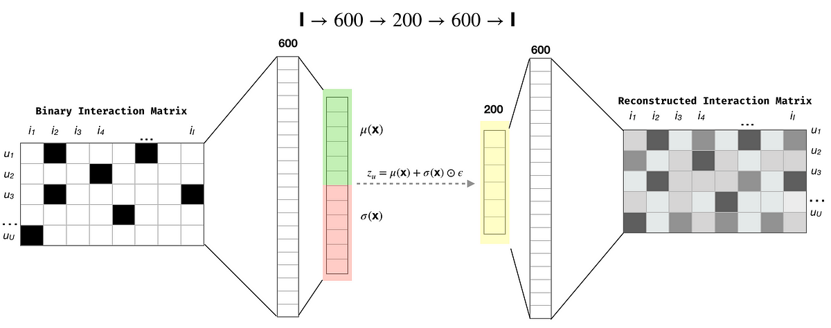
Let me first describe the notational convention. Following Liang et al., 2018, I will use u ∈ {1,…,U} to index users and i ∈ {1,…,I} to index items. The user-by-item binary interaction matrix (i.e. the click matrix) is X ∈ ℕ^{U × I} and I will use lower case xᵤ =[X{u1},…,X{uI}] ∈ ℕ^I to refer to the click history of an individual user u.

With that notation, the Mult-VAE Loss function is defined as:

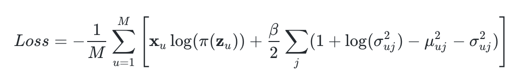
where M is the mini-batch size. The first element within the summation is simply the log-likelihood of the click history _xᵤ **conditioned to the latent representation **z_ᵤ, i.e. log(pθ(xᵤ|z_ᵤ_)) (see below). The second element is the Kullback–Leibler divergence for VAEs when both the encoder and decoder distributions are Gaussians (see here).

We just need a bit more detail before we can jump to the code. xᵤ,the click history of user u, is defined as:

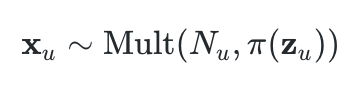
where**_ Nᵤ = ∑ᵢ Nᵤᵢ **is the total number of clicks for user u. As I mentioned before, **z_ᵤ**is latent representation of xᵤ,and is assumed to be drawn from a standard Gaussian prior pθ(**z_ᵤ**)∼ N(0, I). During the implementation of the Mult-VAE, **z_ᵤ **needs to be sampled from an approximate posterior qϕ(**z_ᵤ∣x_ᵤ**​) (which is also assume to be Gaussian). Since computing gradients when sampling is involved is…“complex”, Kingma and Welling introduced the so-called reparameterization trick (please, read the original paper, original post, or any of the multiple online resources.) for more details on the reparameterization trick), so that the sampled **z_ᵤ _**will be computed as:

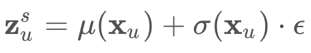
μ and σ in Eq 3 are functions of neural networks and ϵ ∼ N(0, I) is Gaussian noise. Their computation will become clearer later in the post when we see the corresponding code. Finally, π(z_ᵤ_) in Eq (2) is π(z_ᵤ_)= Softmax(z_ᵤ_).

At this stage we have almost all the information we need to implement the Mult-VAE and its loss function in Eq (1): we know what **_xᵤ _**is, **z_ᵤ, μ and σ _**will be functions of our neural networks, and π is just the Softmax function. The only “letter” left to discuss from Eq (1) is β.

Looking at the loss function in Eq (1) within the context of VAEs, we can see that the first term is the “reconstruction loss”, while the KL divergence​ act as a regularizer. With that in mind, Liang et al add a factor β to control the strength of the regularization, and propose β<1. For a more in-depth refection of the role of _β, and in general a better explanation of the form of the loss function for the Mult-VAE, _please read the original paper or the original post.

Without further ado, let’s move to the code:

#pytorch #mxnet #variational-autoencoder #recommendation-system #python