This is the sixth article in my series on Reinforcement Learning (RL). We now have a good understanding of the concepts that form the building blocks of an RL problem, and the techniques used to solve them. We have also taken a detailed look at two Value-based algorithms — Q-Learning algorithm and Deep Q Networks (DQN), which was our first step into Deep Reinforcement Learning.

In this article, we will continue our Deep Reinforcement Learning journey and learn about our first Policy-based algorithm using the technique of Policy Gradients. We’ll go through the REINFORCE algorithm step-by-step, so we can see how it contrasts with the DQN approach.

Here’s a quick summary of the previous and following articles in the series. My goal throughout will be to understand not just how something works but why it works that way.

1. Intro to Basic Concepts and Terminology (What is an RL problem, and how to apply an RL problem-solving framework to it using techniques from Markov Decision Processes and concepts such as Return, Value, and Policy)
2. Solution Approaches(Overview of popular RL solutions, and categorizing them based on the relationship between these solutions. Important takeaways from the Bellman equation, which is the foundation for all RL algorithms.)
3. Model-free algorithms_ (Similarities and differences of Value-based and Policy-based solutions using an iterative algorithm to incrementally improve predictions. Exploitation, Exploration, and ε-greedy policies.)_
4. Q-Learning_ (In-depth analysis of this algorithm, which is the basis for subsequent deep-learning approaches. Develop intuition about why this algorithm converges to the optimal values.)_
5. Deep Q Networks(Our first deep-learning algorithm. A step-by-step walkthrough of exactly how it works, and why those architectural choices were made.)
6. Policy Gradient _— this article _(Our first policy-based deep-learning algorithm.)
7. Actor-Critic (Sophisticated deep-learning algorithm which combines the best of Deep Q Networks and Policy Gradients.)
8. Surprise Topic 😄 (Stay tuned!)

If you haven’t read the earlier articles, it would be a good idea to read them first, as this article builds on many of the concepts that we discussed there.

Policy Gradients

With Deep Q Networks, we obtain the Optimal Policy indirectly. The network learns to output the Optimal Q values for a given state. Those Q values are then used to derive the Optimal Policy.

Because of this, it needs to make use of an implicit policy so that it can train itself eg. it uses an ε-greedy policy.

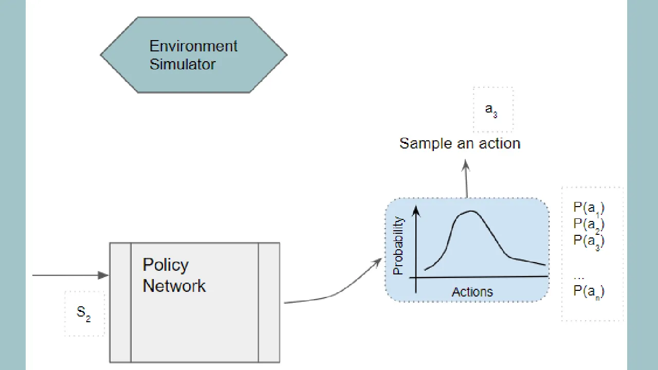
On the other hand, we could build a neural network that directly learns the Optimal Policy. Rather than learning a function that takes a state as input and outputs Q values for all actions, it instead learns a function that outputs the best action that can be taken from that state.

More precisely, rather than a single best action, it outputs a probability distribution of the actions that can be taken from that state. An action can then be chosen by sampling from the probability distribution.

#reinforcement-learning #deep-learning #machine-learning #artificial-intelligence