How the Machine Learns?

Machine learning (ML) is the study of computer algorithms that improve automatically through experience. It is seen as a subset of _artificial intelligence. Machine learning algorithms build a mathematical model based on sample data, known as “training data”, in order to make predictions or decisions without being explicitly programmed to do so.

We, as humans can study data to find the behavior and predict something based on the behavior, but a machine can’t really operate like us. So, in most cases, it tries to learn from already established examples. Say, for a classic classification problem, we have a lot of examples from which the machine learns. Each example is a particular circumstance or description which is depicted by a combination of features and their corresponding labels. In our real-world, we have a different description for every different object and, we know these different objects by different names. For example, cars and bikes are just two object names or two labels. They have different descriptions like the number of wheels is two for a bike and four for a car. So, the number of wheels can be used to differentiate between a car and a bike. It can be a feature to differentiate between these two labels.

Every common aspect of the description of different objects which can be used to differentiate it from one another is fit to be used as a feature for the unique identification of a particular object among the others. Similarly, we can assume, the age of a house, the number of rooms and the position of the house will play a major role in deciding the costing of a house. This is also very common in the real world. So, these aspects of the description of the house can be really useful for predicting the house price, as a result, they can be really good features for such a problem.

In machine learning, we have mainly two types of problems, classification, and regression. The identification between a car and a bike is an example of a classification problem and the prediction of the house price is a regression problem.

We have seen for any type of problem, we basically depend upon the different features corresponding to an object to reach a conclusion. The machine does a similar thing to learn. It also depends on the different features of objects to reach a conclusion. Now, in order to differentiate between a car and a bike, which feature will you value more, the number of wheels or the maximum speed or the color? The answer is obviously first the number of wheels, then the maximum speed, and then the color. The machine does the same thing to understand which feature to value most, it assigns some weights to each feature, which helps it understand which feature is most important among the given ones.

Now, it tries to devise a formula, like say for a regression problem,

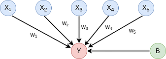
Equation 1

Here w1,w2, w3 are the weights of there corresponding features like x1,x2, x3 and b is a constant called the bias. Its importance is that it gives flexibility. So, using such an equation the machine tries to predict a value y which may be a value we need like the price of the house. Now, the machine tries to perfect its prediction by tweaking these weights. It does so, by comparing the predicted value y with the actual value of the example in our training set and using a function of their differences. This function is called a loss function.

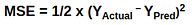
Equation 2

The machine tries to decrease this loss function or the error, i.e tries to get the prediction value close to the actual value.

Gradient Descent

This method is the key to minimizing the loss function and achieving our target, which is to predict close to the original value.

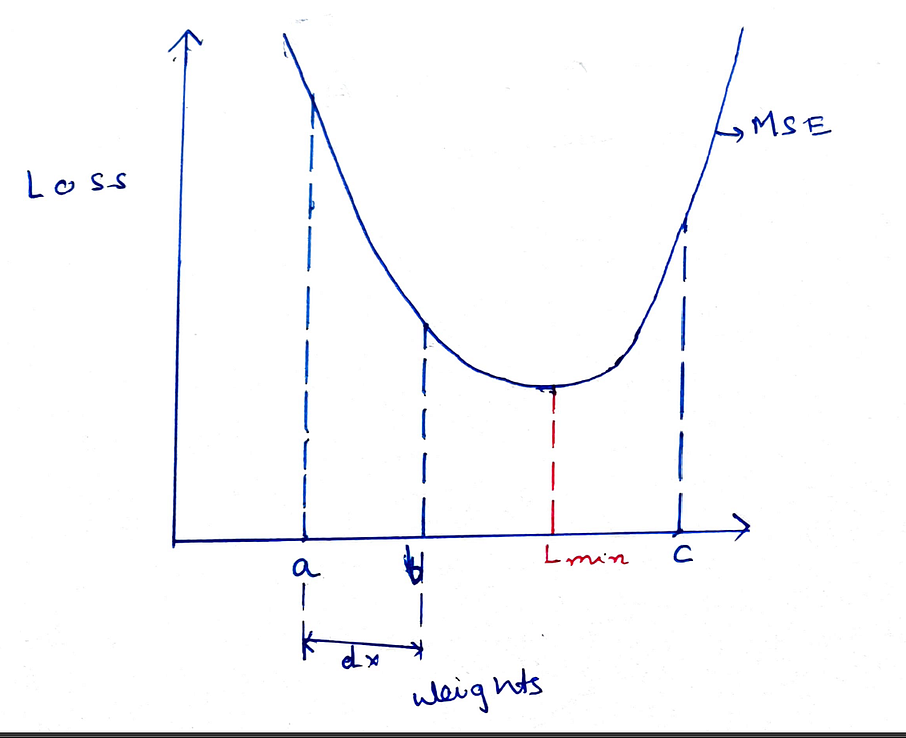
Gradient descent for MSE

In this diagram, above we see our loss function graph. If we observe we will see it is basically a parabolic shape or a convex shape, it has a specific global minimum which we need to find in order to find the minimum loss function value. So, we always try to use a loss function which is convex in shape in order to get a proper minimum. Now, we see the predicted results depend on the weights from the equation. If we replace equation 1 in equation 2 we obtain this graph, with weights in X-axis and Loss on Y-axis.

Initially, the model assigns random weights to the features. So, say it initializes the weight=a. So, we can see it generates a loss which is far from the minimum point L-min.

Now, we can see that if we move the weights more towards the positive x-axis we can optimize the loss function and achieve minimum value. But, how will the machine know? We need to optimize weight to minimize error, so, obviously, we need to check how the error varies with the weights. To do this we need to find the derivative of the Error with respect to the weight. This derivative is called Gradient.

Gradient = dE/dw

Where E is the error and w is the weight.

Let’s see how this works. Say, if the loss increases with an increase in weight so Gradient will be positive, So we are basically at the point C, where we can see this statement is true. If loss decreases with an increase in weight so gradient will be negative. We can see point A, corresponds to such a situation. Now, from point A we need to move towards positive x-axis and the gradient is negative. From point C, we need to move towards negative x-axis but the gradient is positive. So, always the negative of the Gradient shows the directions along which the weights should be moved in order to optimize the loss function. So, this way the gradient guides the model whether to increase or decrease weights in order to optimize the loss function

#neural-networks #backpropagation #machine-learning #gradient-descent