This tutorial was supposed to be published last week. Except I couldn’t get a working (and decent) model ready in time to write an article about it. In fact, I’ve had to spend 2 days on the code to wrangle some semblance of useful and legible output from it.

But I’m not mad at it (now). This is the aim of my challenge here and truthfully I was getting rather tired of solving all the previous classification tasks in a row. And the good news is I’ve learned how to model the data in a suitable format for processing, conducting exploratory data analysis on time-series data and building a good (the best I could come up with, like, after 2 days) model.

So I’ve also made a meme to commemorate my journey. I promise the tutorial is right on the other side of it.

Yes, I made a meme of my own code.

_About the Dataset: __The Gas Sensor Array Dataset, download from here**, _**consists of 8 sensor readings all set to detect concentration levels of a mixture of Ethylene gas with either Methane or Carbon Monoxide. The concentration levels are constantly changing with time and the sensors record this information.

Regression is one other possible type of solution that can be implemented for this dataset, but I deliberately chose to build a multivariate time-series model to familiarize myself with time-series forecasting problems and also to set more of a challenge to myself.

Time-Series data continuosuly varies with time. There may be one variable that does so (univariate), or multiple variables that vary with time (multivariate) in a given dataset.

Here, there are 11 feature variables in total; 8 sensor readings (time-dependent), Temperature, Relative Humidity and the Time (stamp) at which the recordings were observed.

As with most datasets in the UCI Machine Learning Repository, you will have to spend time cleaning up the flat files, converting them to a CSV format and insert the column headers at the top.

If this sounds exhausting to you, you can simply downloadone such file I’ve already prepped.

---

T

his is going to be a long tutorial with explanations liberally littered here and there, in order to explain concepts that most beginners might not be knowing. So in advance, thank you for your patience and I’ll keep the explanations to the point and as short as possible.

1) Exploratory Data Analysis -

Before heading into the data preprocessing part, it is important to visualize what variables are changing with time and how they are changing (trends) with time. Here’s how.

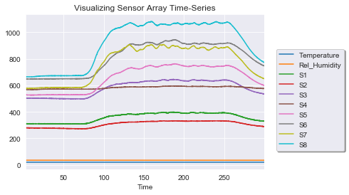
Time Series Data Plot

# Gas Sensing Array Forecast with VAR model

	# Importing libraries
	import numpy as np, pandas as pd
	import matplotlib.pyplot as plt, seaborn as sb

	# Importing Dataset
	df =  pd.read_csv("dataset.csv")
	ds = df.drop(['Time'], axis = 1)

	# Visualize the trends in data
	sb.set_style('darkgrid')
	ds.plot(kind = 'line', legend = 'reverse', title = 'Visualizing Sensor Array Time-Series')
	plt.legend(loc = 'upper right', shadow = True, bbox_to_anchor = (1.35, 0.8))
	plt.show()

	# Dropping Temperature & Relative Humidity as they do not change with Time
	ds.drop(['Temperature','Rel_Humidity'], axis = 1, inplace = True)

	# Again Visualizing the time-series data
	sb.set_style('darkgrid')
	ds.plot(kind = 'line', legend = 'reverse', title = 'Visualizing Sensor Array Time-Series')
	plt.legend(loc = 'upper right', shadow = True, bbox_to_anchor = (1.35, 0.8))
	plt.show()
view raw
gsr_data_prepocessing.py hosted with ❤ by GitHub

It is evident that the ‘Temperature’ and ‘Relative Humidity’ variables do not really change with time at all. Therefore I have dropped the columns; time, temperature and rel_humidity from the dataset, to ensure that it only contains pure, time-series data.

2) Checking for Stationarity:

Non-stationary data has trends that are present in the data. We will have to eliminate this property because the Vector Autoregression (VAR) model, requires the data to be stationary.

A Stationary series is one whose mean and variance do not change with time.

One of the ways to check for stationarity is the ADF test. The ADF test has to be implemented for all the 8 sensor readings column. We’ll also split the data into train & test subsets.

#multivariate-analysis #time-series-forecasting #data-science #machine-learning #time-series-analysis #data analysis