A time series is a sequence of data samples taken in time order with equal time intervals. Time series include many kinds of real experimental data taken from various domains such as finance, medicine, scientific research (e.g., global warming, speech analysis, earthquakes), etc. [1][2]. Time series forecasting has many real applications in various areas such as forecasting of business (e.g., sales, stock), weather, decease, and others [1].
Given a traditional (time order independent) dataset for supervised machine learning for prediction, data exploration and preprocessing are required before features engineering can be performed, and the features engineering needs to be done before a machine learning model can be chosen and applied to the engineered features for prediction.
Similarly to traditional dataset, given a time series dataset, data exploration and preprocessing are required before the time series data can be analyzed, and time series data analysis is required before a time series forecasting model can be chosen and applied to the analyzed dataset for forecasting.
In this article, I use a global warming dataset from Kaggle [2] to demonstrate some of the common time series data preprocessing/analysis methods and time series forecasting models in Python. The demonstration consists of the following:
- Time series data preprocessing
- Time series data analysis
- Time series forecasting
1. Time Series Data Preprocessing
As described before, for a time series data, data preprocessing is required before data analysis can be performed.
1.1 Loading Data
The first step towards data preprocessing is to load data from a csv file.
Time order plays a critical role in time series data analysis and forecasting. In particular, each data sample in a time series must be associated with a unique point in time. This can be achieved in Pandas DataFrame/Series by using values of DatetimeIndex type as its index values.
Once the earth surface temperature dataset in Kaggle [2] has been downloaded onto a local machine, the dataset csv file can be loaded into a Pandas DataFrame as follows:
df_raw = pd.read_csv('./data/GlobalTemperatures.csv', parse_dates=['dt'], index_col='dt')
df_raw.head()
The option parse_dates is to tell Pandas to parse the string values in the_ dt _column into Python _datatime _values, while the option index_col is to tell Pandas to convert the parsed values of the _dt _column into DatatimeIndex type and then use them as indices.
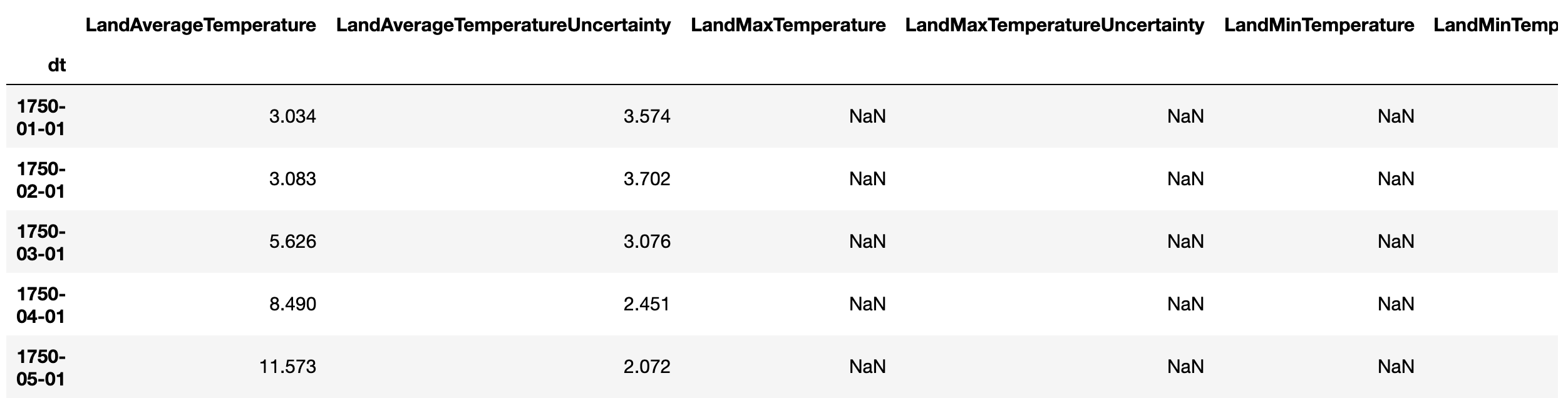
For simplicity, I extract the LandAverageTemperature column as a Pandas Series for demonstration purpose in this article:
df = df_raw['LandAverageTemperature']
1.2 Handling Missing Data
Similarly to a traditional dataset, missing data frequently occurs in time series data, which must be handled before the data can be further preprocessed and analyzed.
The following code can check how many data entries are missing:
df.isnull().value_counts()
There are 12 missing data entries in the earth surface temperature time series. Those missing values cannot simply be removed or set to zero without breaking the past time dependency. There are multiple ways of handling missing data in time series appropriately [3]:
- Forward fill
- Backward fill
- Linear interpolation
- Quadratic interpolation
- Mean of nearest neighbors
- Mean of seasonal couterparts
I used forward fill to fill up the missing data entries in this article:
df = df.ffill()
2. Time Series Data Analysis
Once the data preprocessing is done, the next step is to analyze data.
2.1 Visualizing Data
As a common practice [1][3][4], the first step towards time series data analysis is to visualize the data.
The code below uses the Pandas DataFrame/Series built-in plot method to plot the earth surface temperature time series:
ax = df.plot(figsize=(16,5), title='Earth Surface Temperature')
ax.set_xlabel("Date")
ax.set_ylabel("Temperature")
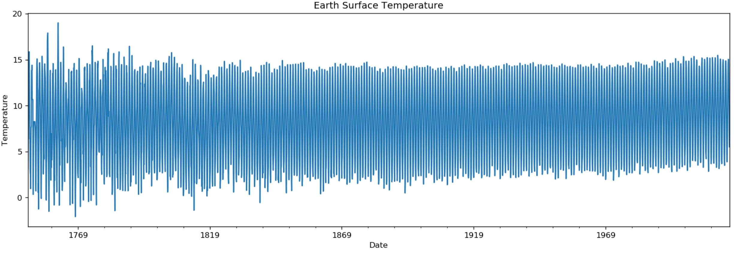
Figure 1: Earth surface temperature.
The above plot shows that the average temperature of the earth’s surface is around the range of [5, 12] and the overall trend is increasing slowly. No other obvious patterns show up in the plot due to mixture of different time series components such as base level, trend, seasonality, and other components such as error and random noise [1][3]. The time series can be decomposed into individual components for further analysis.
2.2 Decomposing Data into Components
To decompose a time series into components for further analysis, the time series can be modeled as an additive or multiplicative of base level, trend, seasonality, and error (including random noise) [3]:
- Additive time series:
- value = base level + trend + seasonality + error
- Multiplicative time series:
- value = base level x trend x seasonality x error
The earth surface temperature time series is modeled as an additive time series in this article:
additive = seasonal_decompose(df, model='additive', extrapolate_trend='freq')
The option extrapolate_trend='freq' is to handle any missing values in the trend and residuals at the beginning of the time series [3].
In theory, the same dataset can be easily modeled as a multiplicative time series by replacing the option _model=’additive’ _with _model=’multiplicative’. _However, the multiplicative model cannot be applied to this particular dataset because the dataset contains zero and/or negative values, which are not allowed in multiplicative seasonality decomposition.
#lstm #data-science #arima #data analysis #data analysis