This article breaks down the topic of support vector machines deductively, covering the most basic approach to the underlying mathematics. The information is supported by examples and aims to create their own approaches to the subject, regardless of their level of knowledge.
Table of Contents (TOC)
1\. Introduction
2\. Kernelized Support Vector Machines
2.1\. Linear Model
2.2\. Polynomial Kernel
2.3\. Gaussian RBF Kernel
3\. Hyperparameters
4\. Under the Hood
1. Introduction
Support Vector Machines are powerful and versatile machine learning algorithms that can be used for both classification and regression. The usage area of these algorithms is quite wide. It is dynamically developed and used in many fields from images classification to medical image cancer diagnosis, from text data to bioinformatics. Since we’re going to take the whole thing and break it down, let’s first illustrate the instinctive basic working of support vector machines.
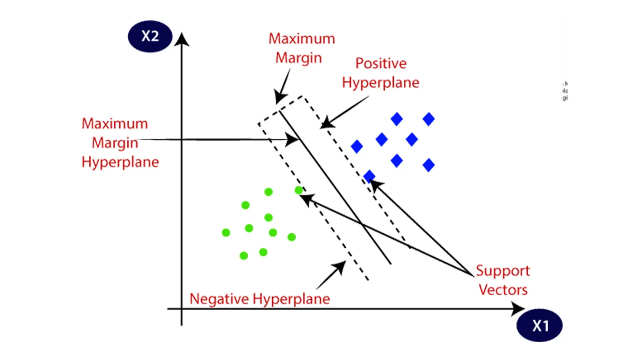
Let’s create a dataset with 2 inputs (x1 and x2) and 2 outputs (purple and red) as seen in figure 1(left). The goal of the model is to predict the class of data which is given x1 and x2 values after the model is trained. In other words, model should distinguish the dataset in the most optimal way. Purple and red data can be linearly separated by an infinite number of linear lines as seen in figure 1(middle). Looking at these lines, it is realized that none of these infinitely drawn points are related to the number or density of data in the dataset. These reference points are called support vectors (Figure 1. right). Support vectors are the data which are closest the hyperplane. Now, let’s quickly separate the make_blob dataset with 100 data and 2 classes, which we imported with the scikit learn library, with the support vector machine.
import mglearn
import matplotlib.pyplot as plt
from sklearn.datasets import make_blobs
import numpy as np
IN[1]
x, y = make_blobs(n_samples=100, centers=4, cluster_std=0.8, random_state=8)
y=y%2
IN[2]
mglearn.discrete_scatter(x[:, 0], x[:, 1], y)
IN[3]
from sklearn.svm import LinearSVC
linear_svm = LinearSVC().fit(x, y)
mglearn.plots.plot_2d_separator(linear_svm, x)
mglearn.discrete_scatter(x[:, 0], x[:, 1], y)
plt.xlabel("Feature 0")
plt.ylabel("Feature 1")
IN[4]
from sklearn.svm import SVC
svm = SVC(kernel='rbf').fit(x, y)
mglearn.plots.plot_2d_separator(svm, x)
mglearn.discrete_scatter(x[:, 0], x[:, 1], y)
plt.xlabel("Feature 0")
plt.ylabel("Feature 1")
It can be seen both in the accuracy of the test data and visually that Linear SVM separates classes worse than the Radial Basis Function (RBF) Kernel. Now let’s examine the kernel types in the Support Vector Machines one by one.
#supervised-learning #artificial-intelligence #data-science #machine-learning