The Neural Network has been developed to mimic a human brain. Though we are not there yet, neural networks are very efficient in machine learning. It was popular in the 1980s and 1990s. Recently it has become more popular. Computers are fast enough to run a large neural network in a reasonable time. In this article, I will discuss how to implement a neural network.

I recommend that you please read this ‘Ideas of Neural Network’ portion carefully. But if it is not too clear to you, do not worry. Move on to the implementation part. I broke it down in even smaller pieces there.

How A Neural Network Works

In a simple neural network, neurons are the basic computation units. They take the input features and channel them out as output. Here is how a basic neural network looks like:

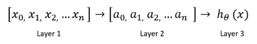
Here, ‘layer1’ is the input feature. ‘Layer1’ goes into another node layer2 and finally outputs the predicted class or hypothesis. Layer2 is the hidden layer. You can use more than 1 hidden layer.

You have to design your neural network based on your dataset and accuracy requirements.

Forward Propagation

The process of moving from layer1 to layer3 is called the forward propagation. The steps in the forward-propagation:

1. Initialize the coefficients theta for each input feature. Suppose, there are 10 input features. Say, we have 100 training examples. That means 100 rows of data. In that case, the size of our input matrix is 100 x 10. Now you determine the size of your theta1. The number of rows needs to be the same as the number of input-features. In this example, that is 10. The number of columns should be the size of the hidden layer which is your choice.
2. Multiply input features X with corresponding thetas and then add a bias term. Pass the result through an activation function.

There are several activation functions available such as sigmoid, tanh, relu, softmax, swish

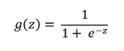
I will use a sigmoid activation function for the demonstration of the neural network.

Here, ‘a’ represents the hidden layer or layer2 and b is the bias.

g(z) is the sigmoid activation:

3. Initialize theta2 for the hidden layer. The size will be the length of the hidden layer by the number of output classes. In this example, the next layer is the output layer as we do not have any more hidden layers.

4. Then we need to follow the same process as before. Multiply theta and the hidden layer and pass through the sigmoid activation layer to get the hypothesis or predicted output.

Backpropagation

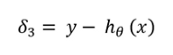
Backpropagation is the process of moving from the output layer to layer2. In this process, we calculate the error.

1. First, subtract the hypothesis from the original output y. That will be our delta3.

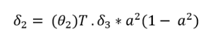
2. Now, calculate the gradient for theta2. Multiply delta3 to theta2. Multiply that to ‘a2’ times ‘1- a2’. In the formula below superscript 2 on ‘a’ represents the layer2. Please do not misunderstand it as a square.

3. Calculate the unregularized version of the gradient from diving delta by the number of training examples m.

#machine-learning #artificial-intelligence #neural-networks #deep-learning #towards-ai #deep learning