SVM is a very simple yet powerful supervised machine learning algorithm that can be used for classification as well as regression though its popularly used for classification. They perform really well in small to medium sized datasets and are extremely easy to tune.
In this blog post we will build our intuition of support vector machines and see some math behind it. We will first understand what large margin classifiers are and understand the loss function and the cost function of this algorithm. We will then see how regularization works for SVM and what governs the bias/variance trade off. Finally we will learn about the coolest feature of SVM, that is the Kernel trick.
You must have some pre-requisite knowledge of how linear regression and logistic regression work in order to easily grasp the concepts. I would suggest you to take notes while reading in order to make the most out of this article, it is going to be a long and interesting journey. So, without further ado lets dive in.
Large Margin Classifier
Lets right away begin with an example, say we have some data which contains 2 classes and for simplicity lets assume it has only 2 features, we can separate these 2 classes in many different ways. We can use linear as well as non-linear decision boundaries to do so.
What SVM does is that it tries to separate these 2 classes as widely as possible and hence in our example it will choose the yellow line as its decision boundary.
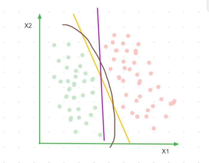
Figure 1
If the yellow line is our decision boundary then the green and red class points circled (figure 2) are the closest points to our decision boundary. The distance between these points is called margin and SVM tries to maximize this margin. This is the reason why support vector machines are also called **large margin classifiers, **this enables SVM to have a better generalization accuracy.
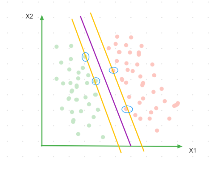
Figure 2
In high dimensional space these points are nothing but n-dimensional vectors where n is the number of features in the data. A sample of points that are closest to the decision boundary (here the circled red and green points) are called support vectors. I will be calling the green support vectors as positive support vectors and the red as negative support vectors. The decision boundary is entirely dependent on these points as they are the ones which decide the length of our margin. If we change the support vectors, our decision boundary will change and that also means that points other than the support vectors don`t really matter in forming our decision boundary.
Optimization Objective
To find the decision boundary we must :
- define our hypothesis
- define a loss function
- using the loss function calculate the cost function for all the training points
- use an optimization algorithm like gradient descent or sequential minimal optimization to minimize the cost and arrive at our ideal parameters
The hypothesis for SVM is fairly straight forward, for weights w
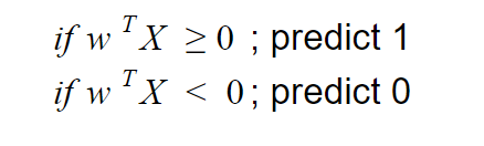
Figure 3
Here a key point that you need to understand is that this hypothesis is nothing but the distance between a data point and the decision boundary, so whenever I say the word hypothesis just think of it as nothing but this distance .
Before we see what exactly the loss function is for SVM let us look at the cost for a single training example
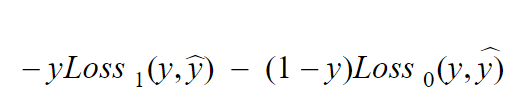
Figure 4
The first term is the loss for when y = 1 and the second term is the loss when y = 0 and “y hat” is nothing but our hypothesis defined in Figure 3. I know I have given out a lot of equations dont worry, lets start making sense out of them.
#algorithms #classification #machine-learning #data-science #support-vector-machine #algorithms