Abstract

In this blog post, we present a formal treatment of receptive fields of convolution layers and characterizations of multi-scale convolutional feature maps using a derived mathematical framework. Using the developed mathematical framework, we compute the receptive fields and spatial scales of feature maps under different convolutional and pooling operations. We show the significance of pooling operations to ensure the exponential growth of spatial scale of feature maps as a function of layer depths. Also, we observe that without pooling operations embedded into CNNs, feature map spatial scales only grow linearly as layer depth increase. We introduce spatial scale profile as the layer-wise spatial scale characterization of CNNs which could be used to assess the compatibility of feature maps with histograms of object dimensions in training datasets. This use case is illustrated by computing the spatial scale profile of ResNet-50. Also, we explain how feature pyramid module generates multi-scale feature maps enriched with augmented semantic representations. Finally, it is shown while dilated convolutional filters preserve the spatial dimensions of feature maps, they maintain greater exponential growth rate of spatial scales compared to their regular convolutional filter counterparts.

_Reading this blogpost, you will have a deeper insight into the intuitions behind the use cases of multi-scale convolutional feature maps in the recent proposed CNN architectures for variety of vision tasks. Therefore, this blogpost can be treated as a tutorial to learn more about how different types of layers impact the spatial scales and receptive fields of feature maps. Also, this blogpost is for those engineers and researchers that are involved in designing CNN architectures and are tired of blind trial and error of which feature maps to choose from a CNN backbone to improve the performance of their models, and instead, prefer from the early steps of design process, to match the spatial scale profiles of feature maps with the object dimensions in training datasets. To facilitate such use cases, we have made our code base publicly available at _https://github.com/rezasanatkar/cnn_spatial_scale.

Introduction

It is a general assumption and understanding that feature maps generated by the early convolutional layers of CNNs encode basic semantic representations such as edges and corners, whereas deeper convolutional layers encode more complex semantic representations such as complicated geometric shapes in their output feature maps. Such a characteristic of CNNs to generate feature maps with multi semantic levels is resultant of their hierarchical representational learning ability which is based on multi-layer deep structures. Feature maps with different semantic levels are critical for CNNs because of the two following reasons: (1) complex semantics feature maps are built on top of basic semantic feature maps as their building blocks (2) a number of vision tasks like instance and semantic segmentation benefit from both basic and complex semantic feature maps. A vision CNN-based architecture takes an image as input, and passes it through several convolutional layers with the goal of generating semantic representations corresponding to the input image. In particular, each convolution layer outputs a feature map, where the extent of the encoded semantics in that feature map depends on both the representational learning ability of that convolutional layer as well as its previous convolutional layers.

CNN Feature Maps are Spatial Variance

One important characteristic of CNN feature maps is that they are spatial variance, meaning that CNN feature maps have spatial dimensions, and a feature encoded by a given feature map might only become active for a subset of spatial regions of the feature map. In order to better understand the spatial variance property of CNN feature maps, first, we need to understand why the feature maps generated by fully connected layers are not spatial variance. The feature maps generated by fully connected layers (you can thinks of the activations of neurons of a given fully connected layer as its output feature map) do not have spatial dimensions since every neuron of a fully connected layer is connected to all the input units of the fully connected layer. Therefore, it is not possible to define and consider a spatial aspect for a neuron activation output.

On the other hand, every activation of a CNN feature map is only connected to a few input units, which are in each other spatial neighborhood. This property of CNN feature maps gives rise to their spatial variance characteristic, and is resultant from the spatial local structure of convolution filters and their spatially limited receptive fields. The differences between fully connected layers and convolutional layers which result in spatial invariance for one and spatial variance for the other one is illustrated in the below image where the input image is denoted by the green rectangle, and the brown rectangle denotes a convolutional feature map. Also, a fully connected layer with two output neurons is denoted by two blue and grey circles. As you can see, each neuron of the fully connected layer is impacted by all the image pixels whereas each entry of feature map is only impacted by a local neighborhood of input pixels.

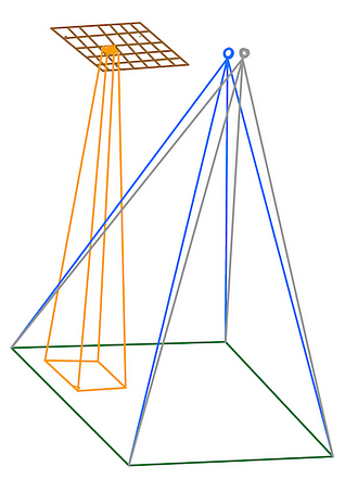
This figure illustrates why the features generated by fully connected layers are not spatial variance while convolutional layers generate spatial variance feature maps. The green rectangle denotes the input image and the brown rectangle denotes a feature map with dimension 5 x 7 x 1 generated by a convolution layer of a CNN. On the other hand, the two blue and grey circles denote activation outputs of a fully connected layer with two output neurons. Let assume the blue neuron (feature) of the fully connected layer will become active if there is a bicycle in the input image while its grey neuron (feature) will become active if there is car in the input image. In other words, the blue neuron is the bicycle feature while the grey neuron is the car feature. Because of the nature of fully connected layers which each neuron’s output is impacted by all the input image pixels, the fully connected layers’ generated features cannot encode any localization information out-of-the-box in order to tell us where in the input image the bicycle is located if there is a bicycle in input image. On the other hand, the feature maps generated by convolutional layers are spatial variance and therefore, they encode the localization information in addition to the existence information of objects. In particular, a generated feature map of dimension W x H x C by a convolutional layer, contains information of existence of C different features (each channel, the third dimension of the feature map, encode existence information of a unique feature) where the spatial dimension W x H of features tell us for which location of the input image, the feature is activated. In this example, the brown convolutional feature map only encodes one feature since it has only one channel (its third dimension is equal to one). Assuming this brown feature map is the bicycle feature map, then an entry of this feature map becomes active only if there is a bicycle in the receptive field of that entry in input image. In other words, this entry does not become active if there is a bicycle in the input image but not in its specific receptive field. Such property of convolutional feature maps enable them not only to encode information about the existence of objects in input images, but also to encode localization information of objects.

#convolutional-network #dilated-convolution #receptive-field #feature-pyramid-network #neural networks