Automated recommender systems are commonly used to provide users with product suggestions that would be of their interest based on existing data about preferences. The literature describes different types of recommender systems. However, we will highlight two major categories and then expand further on the second one:
Content-based filtering: These make use of user preferences in order to make new predictions. When a user provides explicit information about his/her preferences, this is recorded and used by the system to automatically make suggestions. Many of the websites and social media that we commonly use everyday fall into this category.
Collaborative filtering: What happens when there isn’t enough information provided by a user to make item recommendations? Well, in these cases we can use data provided by other users with similar preferences. Methods within this category make use of the history of past choices of a group of users in order to elicit recommendations.
Whereas in the first case it is expected for a given user to build a profile that clearly states preferences, in the second scenario this information may not be fully available, but we expect our system to still be able to make recommendations based on evidence that similar users provide. A method, known as Probabilistic Matrix Factorization, or PMF for short, is commonly used for collaborative filtering, and will be the topic of our discussion for the remainder of this article. Let us now delve into the details of this algorithm as well as its intuitions.
Probabilistic Matrix Factorization Explained
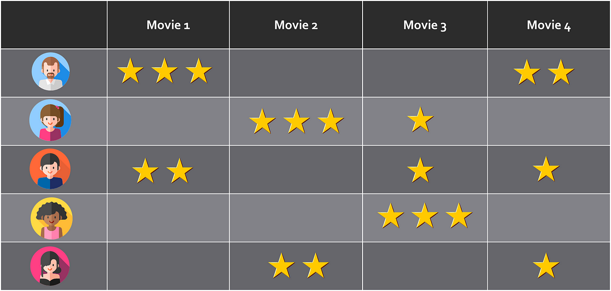
Let’s suppose we have a set of users _u_1, _u_2, _u_3 … _u_N who rate a set of items _v_1, _v_2, _v_3 … _v_M. We can then structure the ratings as a matrix R of N rows and _M _columns, where N is the number of users and M is the number of items to rate.
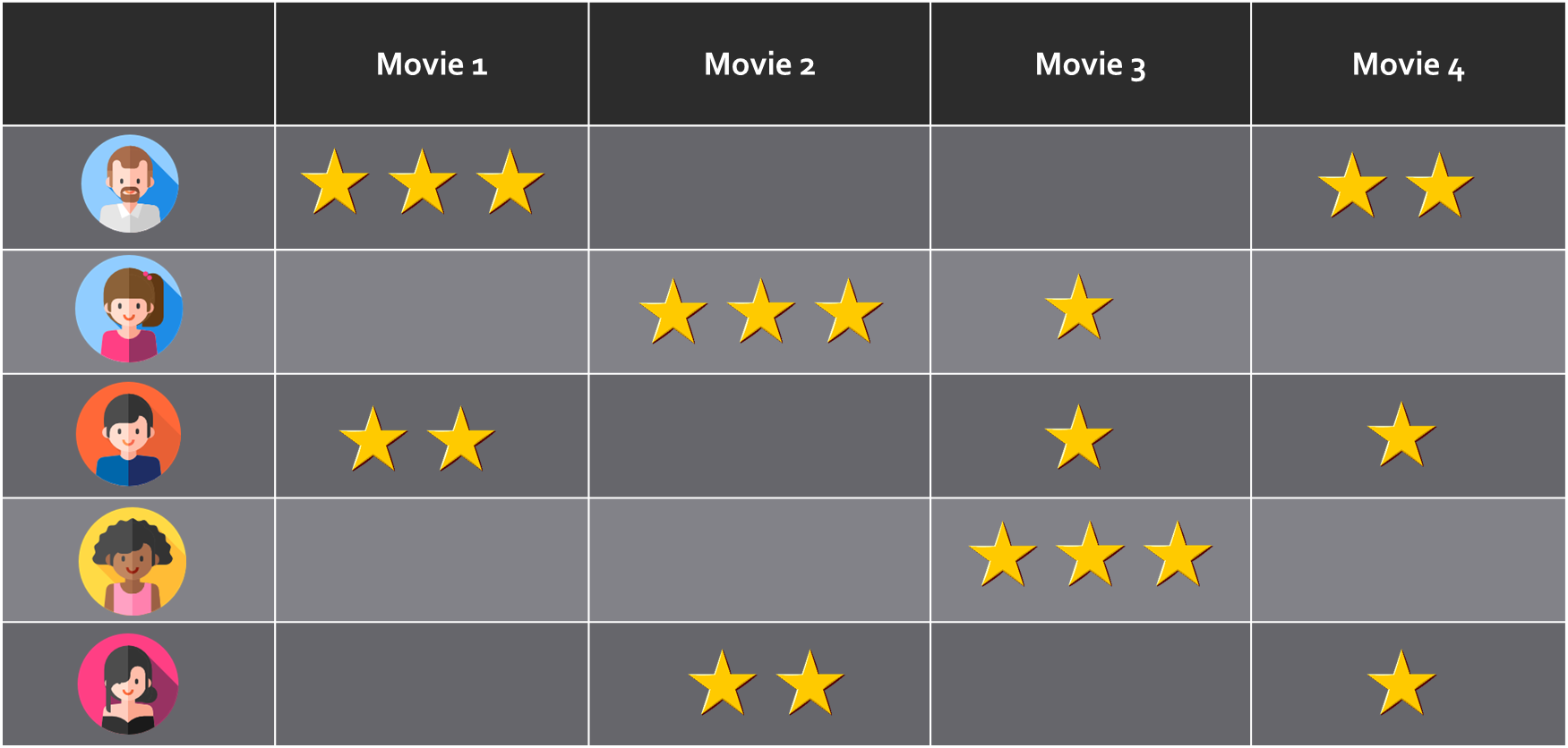
Ratings mapping. It can be thought of as a matrix where each user (rows) rates a number of items (columns)
One important trait of the R matrix is that it is sparse. That is, only some of its cells will have a non-empty rating value, while others will not. For a given user A, the system should be able to offer item recommendations based on his/her preferences as well as the choices made by similar users. However, it is not necessary for user A to have explicitly rated a particular item for it to be recommended. Other users with similar preferences will make up for the missing data about user A. This is why _Probabilistic Matrix Factorization _falls into the category of collaborative filtering recommender systems.
Let’s think for a moment about a recommender system for movies. Imagine what things would be like if we were required to watch and rate every single movie that shows during a particular season. That would be pretty impractical, wouldn’t it? We simply lack the time to do so.
Given that not all users are able to rate all items available, we must find a way to fill in the information gaps of the R matrix and still be able to offer relevant recommendations. PMF tackles this problem by making use of ratings provided by similar users. Technically speaking, it makes use of some principles of Bayesian learning that are also applicable in other scenarios where we have scarce or incomplete data.
The R matrix can be estimated by using two low-rank matrices U and V as shown below:
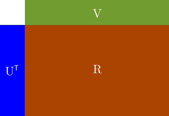
Components of R matrix
Here, **U**T is an N_x_D matrix where N is the number of registered users, and D is the rank. V is a D_x_M matrix, where M is the number of items to rate. Thus the _N_x_M _ratings matrix R can be approximated by means of:
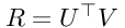
Equation 1: R expression
Our job from now on is to find **U**T and V which in turn, will become the parameters of our model. Because U and V are low-rank matrices, PMF is also known as a low-rank matrix factorization problem. Furthermore, this particular trait of the U and V matrices makes PMF scalable even for datasets containing millions of records.
PMF takes its intuitions from Bayesian learning for parameter estimation. In general, we can say that in Bayesian inference, our aim is to find a posterior distribution of the model parameters by resorting to Bayes rule:
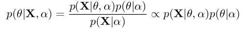
Equation 2: Bayes rule for inference of parameters
Here, X is our dataset, θ is the parameter or parameter set of the distribution. α is the hyperparameter of the distribution. p(θ|X,α) is the posterior distribution, also known as a-posteriori. p(X|θ,α) is the likelihood, and p(θ|α) is the prior. The whole idea of the training process is that as we get more information about the data distribution, we will adjust the model parameter θ to fit the data. Technically speaking, the parameters of the posterior distribution will be plugged into the prior distribution for the next iteration of the training process. That is, the posterior distribution of a given training step will eventually become the prior of the next step. This procedure will be repeated until there is little variation in the posterior distribution p(θ|X,α) between steps.
Now let’s go back to our intuitions for PMF. As we stated earlier, our model parameters will be U and V_, whereas R will be our dataset. Once trained, we will end up with a revised *_R** matrix that will also contain ratings for user-item cells that were originally empty in R. We will use this revised ratings matrix to make predictions.
#bayesian #probabilistic #machine-learning #pmf #deep learning