A Beginner’s Tutorial to Jupyter Notebooks

Use Jupyter Notebooks for interactive Data Science Projects

A Jupyter Notebook is a powerful tool for interactively developing and presenting Data Science projects. Jupyter Notebooks integrate your code and its output into a single document. That document will contain the text, mathematical equations, and visualisations that the code produces directly in the same page.

This step-by-step workflow promotes fast, iterative development since each output of your code will be displayed right away. That’s why notebooks have become increasingly popular over the last several years, especially in Data Science. Kaggle Kernels are almost exclusively made with Jupyter Notebooks these days.

This article is aimed at beginners looking to get started with Jupyter Notebooks. We’ll go through it all end-to-end: Installation, Basic Usage, and how to create an interactive Data Science project!

Setting up a Jupyter Notebook

To get started with Jupyter Notebooks you’ll need to install the Jupyter library from Python. The easiest way to do this is via pip:

pip3 install jupyter

I always recommend using pip3 over pip2 these days since Python 2 won’t be supported anymore starting January 1, 2020.

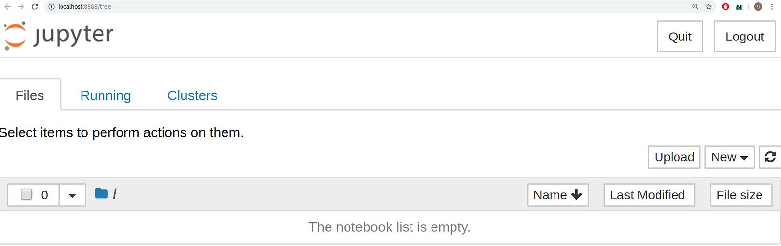
Now that you have Jupyter installed let’s learn how to use it! To get started, use your terminal to move into the folder you would like to work from using the cd command (Linux or Mac). Then start up Jupyter with the following command:

jupyter notebook

This will start up a Jupyter server and your browser will open up a new tab to the following URL: http://localhost:8888/tree. It’ll look a little something like this:

Great! We’ve got our Jupyter server up and running. Now we can start building our notebook and filling it up with code!

The Basics of Jupyter Notebooks

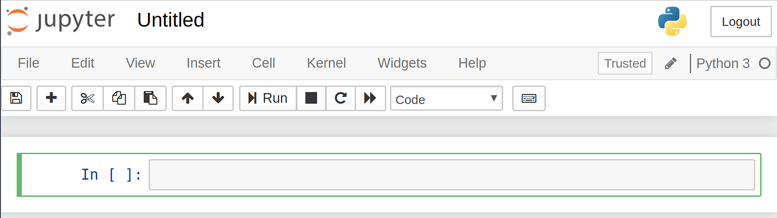
To create a notebook, click on the “new” menu in the top right and select “Python 3”. At this point your web-page will look similar to this:

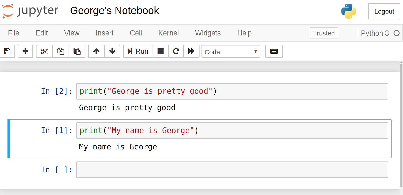
You’ll notice that at the top of your page is the word *Untitled *next to the Jupyter icon — this is the title of your Notebook. Let’s change it to something a little more descriptive. Just move your mouse over the word Untitled and click on the text. You should now see an in-browser dialog where you can rename your Notebook. I’m calling mine George’s Notebook.

Let’s start writing some code!

Notice how the first line of your Notebook is marked with an In [] next to it. That keyword specifies that what you are going to type is an input. Let’s try writing a simply print statement there. Recall that your print statement must have Python 3 syntax since this is a Python 3 Notebook. Once you write your print statement in the cell, press the Run button.

Awesome! See how the output is printed directly on the notebook. This is how we can do an interactive project by seeing the output at each step of the process.

Also notice that when you ran the cell, the first line which had an In [] next to it has now changed to In [1] . The number inside the square brackets indicates the order in which the cell was ran; the first cell has a 1 because it was the first cell that we ran. We can run each cell individually at anytime and those numbers will change.

Let’s take an example.We’re going to set up 2 cells, each one with a different print statement. We’ll run the second print statement first following by the first print statement. Take a look at how the number inside the squared brackets changed as a result.

When you have multiple cells in your Notebook and you run the cells in order, you can share your variables and imports across cells. This makes it easy to separate out your code into related sections without needing to re-create variable at every cell. Just be sure that you run your cells in the proper order so that all your variables are created before usage.

Adding Descriptive Text to Your Notebook

Jupyter Notebooks come with a great set of tools for adding descriptive text to your notebooks. Not only can you write comments, but you can also add titles, lists, bold, and italics. All of this is done in the super easy Markdown format.

The first thing to do is to change the cell type — click the drop down menu that says “Code” on it and change it to “Markdown”. This changes the type of cell we are working with.

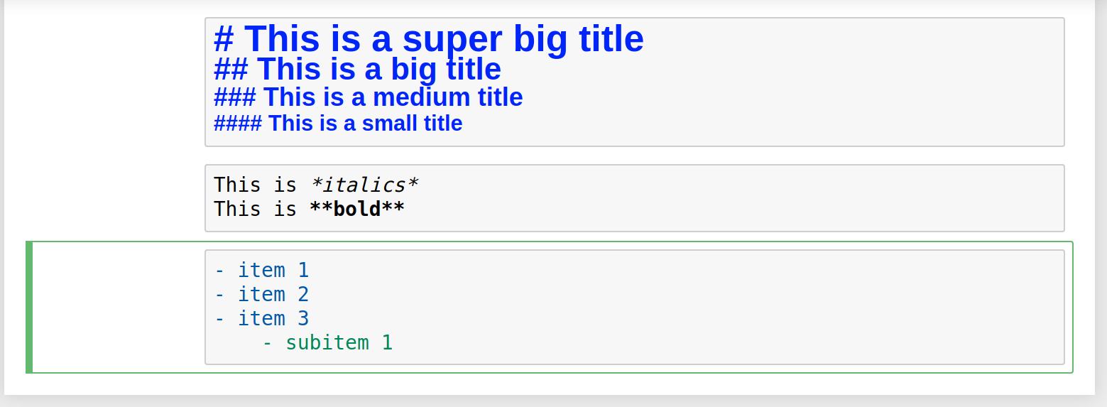
Let’s try out a couple of the options. We can create titles using the # symbol. A single # will make the biggest title and adding more #s will create a smaller and smaller title.

We can italicise our text using a single star on either side or bold it using a double star. Creating a list is easy with a simple dash - and space beside each list item.

Interactive Data Science

Let’s do a quick running example of how to create an interactive Data Science project. This notebook and code comes from an actual project I did.

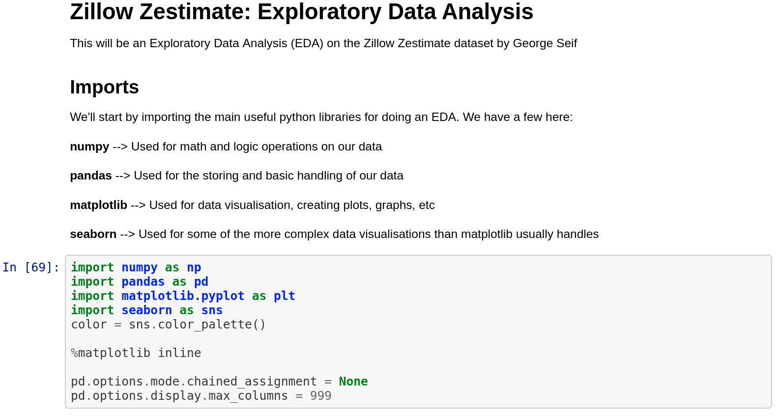
I start out with a Markdown cell and put up a title with the biggest header by using a single # . I then create a list and description of all the important libraries I’m about to import.

Next comes the first code cell which imports all of the relevant libraries. This will be standard Python Data Science code except for 1 additional item: in-order to see your Matplotlib visualisations directly within the notebook, you’ll need to add the following line: %matplotlib inline .

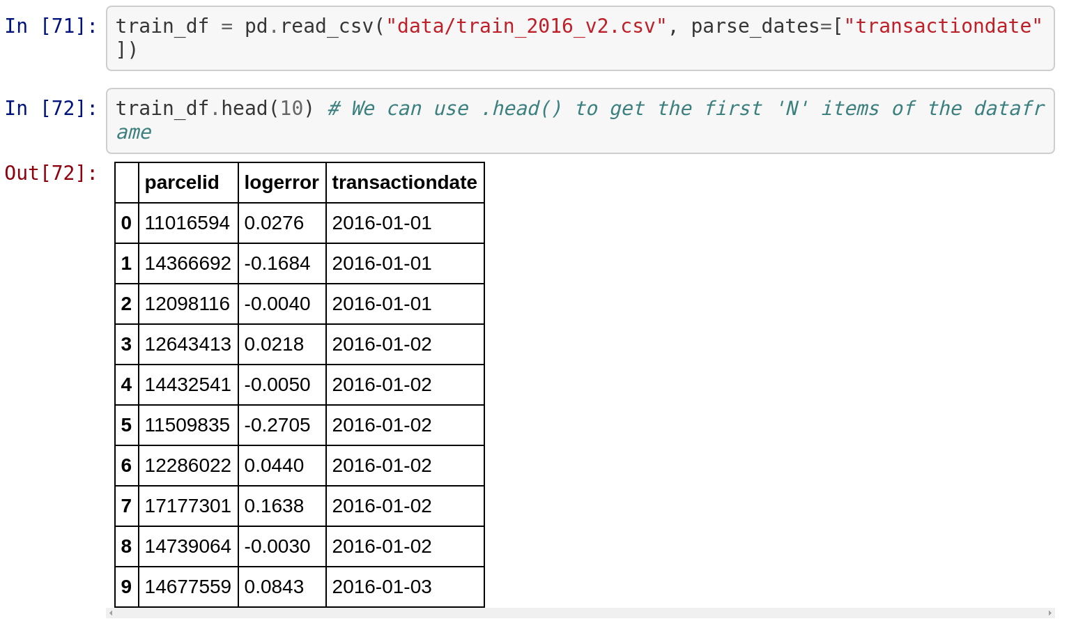
Next I’m going to import a dataset from a CSV file and print out the first 10 items. Notice in the screenshot below how Jupyter automatically shows the .head() function’s output as a table — Jupyter works beautifully with the Pandas library!

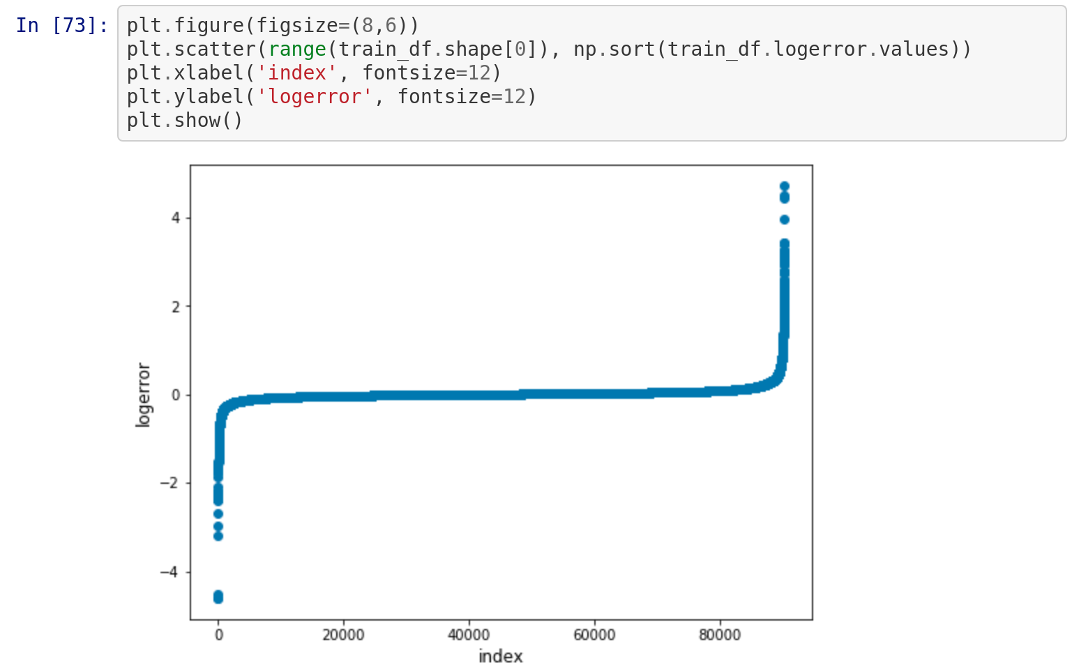
Now we’ll create a figure and plot it directly in our notebook. Since we’ve added the line %matplotlib inline above, anytime we run a plt.show() our figure will be displayed directly in our notebook!

Also notice how all of the variables from previous cells, particularly the dataframe which we read from CSV, carries over to future cells as long as we pressed the “Run” button on those previous cells.

Voila! That’s the easy way to create an interactive Data Science project!

The Menus

The Jupyter server has several menus that you can use to get the most out of your project. These menus enable you to interact with your notebook, as well as access documentation for popular Python libraries and export your project into a format for external presentation.

The File menu allows you to create, copy, rename, and save your notebooks to file. The most notable item in the File menu is the Download as drop down menu which lets you download your notebook in a variety of formats including pdf, html, and slides — perfect for creating a presentation!

The Edit menu lets you do the good’ol can cut, copy, and paste of code. You can also reorder cells here, perhaps if you’re creating a notebook for an interactive presentation and want to show your audience things in a certain order.

The View menu lets you play around with things like displaying line numbers and modifying the toolbar. The best feature in this menu is definitely the Cell Toolbar where you can add tags, notes, and attachments to each cell. You can even select the formatting you would want for this cell if you turned the notebook into a slide show!

The Insert menu is just for inserting cells above or below the currently selected cell. The Cell menu is where you go to run your cells in a specific order or change the cell type.

Finally you have the Help menu which is one of my personal favourites! The help menu gives you direct access to important documentation. You’ll be able to learn about all the Jupyter Notebook shortcuts to speed up your workflow. You also get convenient links to the documentation of some of the most important Python libraries including Numpy, Scipy, Matplotlib, and Pandas!

#data-science #machine-learning #python