Section 0: Introduction

Data imbalance happens when two or more mutually exclusive outcomes of an event occurs with huge difference in frequency. For instance, if your marketing campaign has only 0.001% conversion rate (let’s save quitting the business for another day), then your converted customer VS non-converted traffic is 0.001% VS 99.999%. This is problematic because if you need to predict which customer will likely convert, your model will falsely converge by classifying everything as the majority class. Let’s take a look at my client’s data:

“”
df.shape
df[‘Convert’].value_counts()
“”

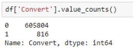
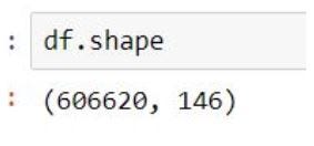
As we can see the data is severely imbalanced with 0.6 million records of “non-adopters” and only 816 rows of “adopters”.

(TL;DR:_ The data has already been cleaned and applied with feature engineering/transformation with different techniques such as Lasso selection, dropping sparse features, Null imputation, etc. Metric was decided to be ROC by the management team. Since this is not our focus in this article, let’s just proceed with the perception that data has been cleaned and goals/metrics are defined.)_

Section 1: Baseline Regular Training

There are lots of solutions out there, and many “mainstream” methodologies have been explored to try to tackle the imbalance issue. By “mainstream” I mean:

• Under-sampling the majority class to make it closer to the rare class (1:1, 1:2, 1:3, 1:5, 1:7… with clustered stratified resampling)
• Over-sampling the rare class with synthetic data (SMOTE, ADASYN, K-means SMOTE…you name it!)
• Duplicating rare class a few times (works amazing on training set but was severely overfitted)
• Giving rare class more weight in models when training

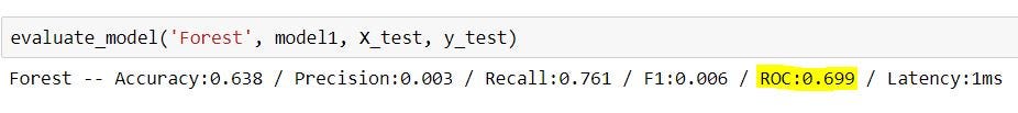
**After splitting training and testing to 80:20 ratio, the best result I could get was by applying under-sampling with 1vs1 class ratio to train RandomForestClassifier(), which means there were around 650 records on each class for training, and around 160 class 1 and 120,000 class 0 in testing set. **The model yields a 69.9% ROC score:

“”
from sklearn.ensemble import RandomForestClassifier
forest = RandomForestClassifier(random_state=5, criterion = ‘entropy’, n_jobs = -1)
model1 = forest.fit(X_train,y_train)

from sklearn.metrics import accuracy_score, precision_score, recall_score, f1_score, roc_auc_score
from time import time
from time import time
def evaluate_model(name, model, features, labels):
start = time()
pred = model.predict(features)
end = time()
accuracy = round(accuracy_score(labels,pred),3)
precision = round(precision_score(labels,pred),3)
recall = round(recall_score(labels,pred),3)
f1 = round(f1_score(labels,pred),3)
roc = round(roc_auc_score(labels,pred),3)

print('{} -- Accuracy:{} / Precision:{} / Recall:{} / F1:{} / ROC:{} / Latency:{}ms'.format(name, accuracy, precision, recall,f1,roc ,round(end-start)))

evaluate_model(‘Forest’, model1, X_test, y_test)
“”

Section 2: Anomaly Detection

The above model did not perform very well, it only trains on ~1300 records and was used to predict 120,000 records. **A lot of information was lost when we reduced class 0 in training set from 480,000 records to just 650 to match the smaller class. **Therefore, Anomaly Detection was explored for our data.

According to the definition, Anomaly Detection trains on majority of the class as “regular events”, and will try to identify the rare events as irregular patterns. It sounds almost like a perfect solution for us, let’s take a look:

First, to avoid “The Curse of Dimensionality”, I applied Kernel Principal Component Analysis (KPCA) to condense the features of the data, and used One-class SVM to train our Anomaly Detection model. By definition, the biggest advantage KPCA has over PCA is its capability of projecting non-linearly-separable data into a high-dimensional space and making data separable.

“”
#Since KPCA requires a lot of memory space, I took a stratified sample
#Splitting the data:

from sklearn.model_selection import train_test_split
X_train, X_test, y_train,y_test = train_test_split(X,y , test_size=0.5, random_state=5, stratify = y)

#scale the data to reduce bias for KPCA:

from sklearn.preprocessing import StandardScaler
scaler = StandardScaler()
trainedscaler = scaler.fit(X_train)
X_train_scaled = trainedscaler.transform(X_train)
X_test_scaled = trainedscaler.transform(X_test)

#Fitting KPCA with only training data to prevent leakage:
from sklearn.decomposition import KernelPCA
kpca = KernelPCA(n_components = 20, n_jobs = -1, kernel = ‘rbf’)
kpcamodel = kpca.fit(X_train_scaled)
X_train_kpca = kpcamodel.transform(X_train_scaled)
X_test_kpca = kpcamodel.transform(X_test_scaled)

#Training model with “majority”, leaving [class 1] out:
train_final = pd.concat([pd.DataFrame(X_train_kpca), y_train], axis =1)
train_0 = train_final[train_final[‘Convert’]==0]
train_1 = train_final[train_final[‘Convert’]==1]

#Prediction:
from sklearn.svm import OneClassSVM
model = OneClassSVM() #again for controlled comparison, no hyperparameters will be tuned
result = model.fit(train_0)
y_pred = result.predict(X_test_kpca)
confusion_matrix(y_train, y_pred)
“”

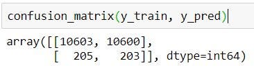
AUC_ROC = 0.5

The model had only 50% on ROC score, which was just random guessing for a binary classifier. I’ve tried multiple iterations with different hyperparameters, nothing could bring the ROC score up by even a few percent, but why….?

Let’s take a look by visualizing the kernel principal components on a 3D graph. The first 3 components explained roughly 64% of the variation:

“”
#Plotting 3D interactive graph with Plotly Express:
import plotly.express as px
plotdata.columns = [“pca0”, ‘pca1’, ‘pca2’, ‘Y’]
fig = px.scatter_3d(plotdata, x=‘pca0’, y=‘pca1’, z=‘pca2’,
color=‘Y’, opacity=0.7)
fig.show()
“”

Created by Author

The yellow dots are converted customers (rare class), the blue dots are non-converted traffic (majority class), the yellow dots perfectly blended in with the blue dots with no distinction, which is clear to us now that** “rare” doesn’t always mean “anomalous”, it could simply mean the data just has smaller quantity, **and therefore,it is not possible for SVM to draw hyperplane between the classes.

According to Dr. Heiko Hoffmann, KPCA and one-class SVM usually produces a very competitive performance. This does not apply to our case because the data’s non-distinguishability demonstrated by the 3D plot above. If the data can be transformed into a linearly-separable space, the results would’ve looked like this:

Left: Original; Upper: PCA; Lower: KPCA; Source: https://rpubs.com/sandipan/197468

To justify my result, I also tried two other Anomaly Detection techniques: Isolation Forest and Local Outlier Factors. It was with no surprise that they didn’t work. While I was a little bummed that Anomaly Detection didn’t work well, I didn’t stop there — there have to be better ways of handling imbalanced data and information loss.

#machine-learning #ensemble-learning #anomaly-detection #data-visualization #data-science