Contrary to popular belief, I hereby state that Logistic Regression is **NOT **a classification algorithm (on its own) — In fact, Logistic Regression is actually a regression model so don’t be surprised “regression” is present in its naming. Regression analysis is a set of statistical process for estimating the relationships between a dependent variable and one or more independent variables (Source: Wikipedia). With that being stated, Logistic regression is empathetically not a classification algorithm — it does not perform statistical classification — since it is simply estimating the parameters of a logistic model.
Logistic Regression is a statistical model that in its most basic form uses a logistic function to model a binary dependent variable, although many more complex extensions exist. (Source: Wikipedia)
What allows Logistic Regression to be used a classification algorithm, as we so commonly do in Machine Learning, is the use of a threshold (may also be referred to as a cut off or decision boundary), which in-turn will classify the inputs with a probability greater than the threshold as one class and probabilities below the threshold as another class._See _this link** to see how we may approach multiclass classification problem.**Now that’s out of the way, let’s revert our attention back to the purpose of the Algorithms from Scratch series.Link to Github Repository…
kurtispykes/ml-from-scratch
Note: There are many Machine Learning frameworks with highly optimized code which makes coding Machine learning algorithms from scratch a redundant task in practical settings. However, when we build algorithms from scratch it helps us to gain a deeper intuition of what is happening in the models which may pay high returns when trying to improve our model.
Linear Regression to Binary Classification
In the last episode of _Algorithms from Scratch: Linear Regression, _I stated “It is usually one of the first algorithms that is learnt when first learning Machine Learning, due to its simplicity and how it builds into other algorithms like Logistic Regression and Neural Networks” — You’ll now see what I meant.How do we go from predicting a continuous variable to Bernoulli variables (i.e. “success” or “failure”)? Well, since the response data (what we are trying to predict) is binary (taking on values 0 and 1), ergo made of only 2 values, we can assume the distribution of our response variable is now from the Binomial distribution — This calls for a perfect time to introduce the Generalized Linear Model (GLM) which was formulated John Nelder and Robert Wedderburn.The GLM model allows for the response variable to have an error distribution other than the normal distribution. In our situation, where we now have a Binomial distribution, by using a GLM model we can generalize linear regression by allowing the linear model to be related to the response variable via a link function and allowing the magnitude of the variance of each measurement to be a function of its predicted value (Source: Wikipedia).
Long story short, Logistic Regression is a special case of the GLM with a binomial conditional response and logit link.
**Halt…**Before going any further we should clear up some statistical terms (In layman’s terms that is):
- **Odds **— The ratio of something happening to something not happening. For instance, the odds of Chelsea FC winning the next 4 games are 1 to 3. The ratio of something happening (Chelsea winning the game) 1 to something not happening (Chelsea not winning the game) 3 can be written as a fraction, 1/3.**Probability **— The ratio of something happening to everything that can happen. Using the example above, the ratio of something happening (Chelsea winning) 1 to everything that can happen (Chelsea winning and losing) 4 can also be written as a fraction 1/4, which is the probability of winning — The probability of losing is therefore 1–1/4 = 3/4.
Probabilities range between 0 and 1, whereas odds are not constrained to be between 0 and 1, but can take any value from 0 to infinity.We can derive the odds from the probability by dividing the ratio of the probability of winning (using our example that would be 1/4) by the ratio of the probability of losing (3/4) which gives us 1/3 — the odds. See Figure 1 for how we can express that mathematically.
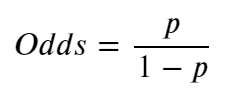
Figure 1: Odds derived from the probability.
If Chelsea were a bad Football Team (Unimaginable, I know) the odds would be against them winning therefore ranging between 0 and 1. However, since we all know that Chelsea is one of the greatest teams in the world (definitely the best in London without a doubt), as a consequence, the odds in favour of Chelsea winning will be between 1 and infinity. The asymmetry makes it difficult to compare the odds for or against Chelsea winning so we take the log of the odds to make everything symmetrical._Figure 1 _shows us that we can calculate the odds with probabilities, that being the case, we can also calculate the log of the odds using the formula presented in Figure 1. The log of the ratio of the probabilities is called the logit function and forms the basis of Logistic Regression. Let’s understand this better by considering a logistic model with given parameters and see how the coefficients can be estimated from the data.
#algorithms-from-scratch #algorithms