How To Effectively Use Geospatial Data in Python

In the geospatial world, the “80% of data is geographic” phrase is commonly used. Although we can’t prove that, lately we see the widespread availability of geospatial data sets.

Handling geographic data is not that easy. It requires domain knowledge to handle geometries and geographic projections. I mainly work with geospatial data. In this article, I’ll show you three ways you can handle geospatial data effectively and quickly in Python.

If you have a data set with latitude and longitude columns, most probably you know you can plot them on a map. But is that it? Do you call it a day and, maybe, explore other nonlocational features?

There is a more systematic and efficient way you can work with geographic data in Python. In this tutorial, I’ll explore how you can efficiently work with location data in Python, enriching your data set and exploring it with specific tools for spatial data in Python.

1. Convert Your Data to GeoDataFrame

First of all, Start converting your data into a GeoDataFrame. So what’s a GeoDataFrame?

If you’re familiar with the Pandas DataFrame, GeoDataFrame is built on top of it with powerfull extra functionalities to handle geographic data.

GeoDataFrame not only offers the flexibility and richness of DataFrame functionality but also has built-in functionality to handle the geometries of your geographic data — hence the name GeoDataFrame.

Converting your data to GeoDataFrame opens up a lot of geographic functionalities that can help you quickly calculate and perform several useful geographic operations on your data.

Some of the functionalities you unlock with converting your data into GeoDataFrame include plotting different maps quickly and integration with other geographic visualisation libraries. Also, It enables performing geometric calculations with one line of code (e.g., buffer, distance, near neighbourhood analysis, etc.).

So let me show an example of how you can convert your Pandas DataFrame into a GeoDataFrame. In this tutorial, we use data sets from the Washington D.C. open-data platform. The nice thing about Open Data DC is it allows you to access the data directly with their APIs without downloading it locally.

# Read in Pandas directly from url source
df = pd.read_csv(‘https://query.data.world/s/6joi7hjgjmwifhl2clpldwm36xmvmx')
# Convert to Geopandas GeoDataFrame
gdf = gpd.GeoDataFrame(df, geometry=gpd.points_from_xy(df.X, df.Y), crs={"init":"epsg:4326"})

In the above code, we first read the data with Pandas and convert it using the GeoPandas method gpd.points_from_xy .gpd.points_from_xy().

By converting your DataFrame to GeoDataFrame, you get an extra geometry column that handles location. Here are the first five rows of gdfGeoDataFrame data.

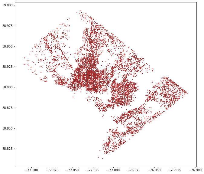
And with GeoPandas, you can plot maps with one line of code:

gdf.plot(ax=ax, markersize=2, color=”brown”)

Map of crimes in Washington D.C.

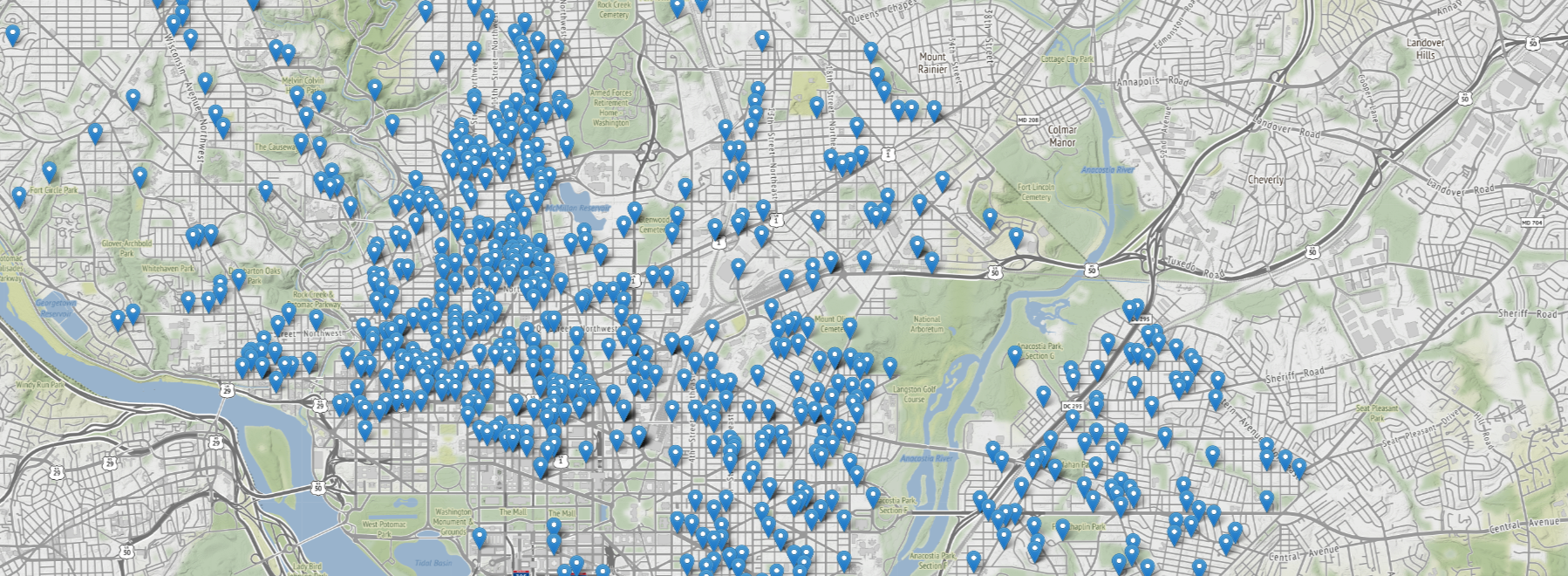
If you want an interactive map with a base map, GeoPandas is integrated well with other geospatial data-visualisation tools in Python.

Let me show you how easy it is to plot the GeoDataFrame into an interactive map with Folium.

m = folium.Map( location=[38.904251, -77.038520], 
                zoom_start=12, tiles=’Stamen Terrain’ )folium.GeoJson( gdf.sample(1000), name=’geojson’).add_to(m)
m

Let me show you an example of some of the functionalities we unlock with this geometry column in the next tip, which will help you understand the coordinate reference system.

2. Know your coordinates

The earth is round, but our maps are flat. The transformation process between the globe into a flat map brings distortions — size, distance, etc. The coordinate reference system (CRS) helps you locate features on the surface of the earth because it gives an original frame of reference for a given data.

Therefore, knowing your CRS is a crucial task in geographic data handling. When you’re performing any geographic operations, take into account the CRS and projection of your data.

If you had paid attention when we converted our DataFrame to a GeoDataFrame, we also provided crs = {"init": “epsg":4326}, and that provides the code for the CRS of the data. This particular code (4326) is for the World Geodetic System (WGS 84), which is widely used for locating the earth. This particular CRS measures in degree units.

There are a lot of CRSs and projections, and finding the right one can be tricky sometimes if you don’t know how to search and find the appropriate one. I usually use EPSG.io to find the correct CRS. You can find measuring units by search by location or even checking EPSG codes if you have one from your data sets.

Having two data sets with different CRSs might not align well once overlayed. That’s one of the most common mistakes in handling geographic data. If your data is not in the right place, start checking your CRS.

But more importantly, the operations carried out with different CRSs have different outputs. Let me show you an example of this by calculating the distance between the centre of Washington D.C. and the crime-point data set we have converted to a GeoDataFrame.

First, let us create a GeoDataFrame out of Washington D.C.’s centre coordinates with the same coordinate reference as the crime data set (epsg:4326).

# City center coordinates
center = Point([-77.036618, 38.907155])
# Create a Geodataframe the center point
center_gdf = gpd.GeoDataFrame(gpd.GeoSeries(center), crs={“init”:”epsg:4326"})
# rename the column to geometry
center_gdf.rename({0:’geometry’}, axis=1, inplace=True)

Now, we can calculate the distance quickly with one line of code, like this:

gdf[‘distance_center’] = gdf.geometry.apply(lambda g: center_gdf.distance(g))
gdf.head()

And here is the output of the first five rows of the data set, including the distance_center calculated above. Have a closer look at these numbers (highlighted in red).

What are those numbers? Can you guess? Feet, meters, kilometres?

Unless you know that epsg:4326 measures its units in degrees, the result might seem weird — or even may mislead you in using these results.

Now, it’s easy to convert to a different projection. Let’s say we want to calculate the distance in meters. When I search “Washington” on the EPSG.io website, I find a lot of CRSs. I pick up this code, epsg:8103, after some research which measures in meters. So let’s see how to project your data into a different CRS in GeoPandas.

# Reproject both datasets-main Geodataframe and center Geodataframe
gdf_proj = gdf.to_crs({‘init’: ‘EPSG:8103’})
center_gdf_proj = center_gdf.to_crs({‘init’: ‘EPSG:8103’})

Let’s recalculate now the distance with this projected data.

gdf_proj[‘distance_center_m’] = gdf_proj.geometry.apply(lambda g: center_gdf_proj.distance(g))
gdf_proj.head()

Have a look at the difference between the last two columns. The last column (highlighted in blue) has distance measured in meters, while the calculated distance in the unprojected data (highlighted in red) is measured in degrees.

Understanding your CRS helps you a lot in dealing with geospatial data. In the next tip, I’ll explore how you can join your data by location and thus enrich your data sets with external data.

3. Enrich your data with spatial join

Feature engineering is an integral part of data preprocessing. However, you see more statistical features like mean and median features often used in augmenting data sets.

Spatial join is often a neglected form of data augmentation that can enrich your data set and bring more features to the dataset.

Let me show you an example here; our data set has crimes and other attributes related to crimes. What if we want to merge another data set — say, poverty rates in the city. I just searched at the DC Open Data portal and found out the poverty areas data set.

The data is not only for our area, but we can filter out to fit our purpose. Let’s read and filter the poverty data set.

poverty = gpd.read_file(“https://opendata.arcgis.com/datasets/5a357128cf2b490e9c716e03dcc03a3e_62.geojson", usecols=[“OBJECTID”,”STATEFP10", “COUNTYFP10”, “TRACTCE10”, “TOTAL_POP”, “UNEMPLOYME”, “POVERTY_RA”, “MEDIAN_INC”, “geometry”])
poverty = poverty[[“OBJECTID”,”STATEFP10", “COUNTYFP10”, “TRACTCE10”, “TOTAL_POP”, “UNEMPLOYME”, “POVERTY_RA”, “MEDIAN_INC”, “geometry”]]
poverty_washington = poverty[poverty[“STATEFP10”] == “11”]
poverty_washington.head()

The poverty table has a few more columns. Still, we filtered out to have only the total population of the area, unemployment, poverty rate, and median income columns. Below are the first few rows of the table:

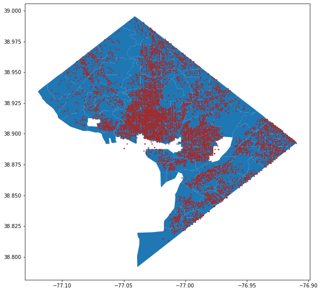
We can overlay both GeoDataFrames (crimes and poverty) onto a map.

fig, ax = plt.subplots(figsize=(12,10))
poverty_washington.plot(column=”COUNTYFP10", ax=ax)
gdf.plot(markersize=2, color=”brown”, ax=ax)
plt.show()

Now, we can carry out aspatial join to merge both data sets by location. But I hope you remember the second tip — check your CRS first before carrying out any geoprocessing task. This time, both data sets have the same CRS.

# Join datasets by location
spatial_join_points = gpd.sjoin(gdf, poverty_washington, op=”within”)
spatial_join_points.head()

Now, we joined the data by location, and that was simple in one line of code. Each point in the crime data set has attributes from the poverty data set now. Let’s look at the first few rows of the spatially joined table.

As you can see, we’ve successfully merged the two data sets based on their location. The spatial join we used is just one method. We performed a within operation to check whether the point is within the polygon. However, there are other operations you can use as well — intersect and contain.

Conclusion

We’ve covered three tips to deal with geospatial data in Python effectively, and that’s just the tip of the iceberg. I couldn’t fit all my favourite tips in this article, but these three tips alone will help you a lot in handling geospatial data.

The code for this article with a Google Collaboratory notebook is available at this GitHub repo.

#python #programming