1. Introduction
1.1. Time-series & forecasting models
Time-series forecasting models are the models that are capable to predict future values based on previously observed values. Time-series forecasting is widely used for non-stationary data. **Non-stationary data **are called the data whose statistical properties e.g. the mean and standard deviation are not constant over time but instead, these metrics vary over time.
These non-stationary input data (used as input to these models) are usually called **time-series. **Some examples of time-series include the temperature values over time, stock price over time, price of a house over time etc. So, the input is a signal (time-series) that is defined by observations taken sequentially in time.
A time series is a sequence of observations taken sequentially in time.
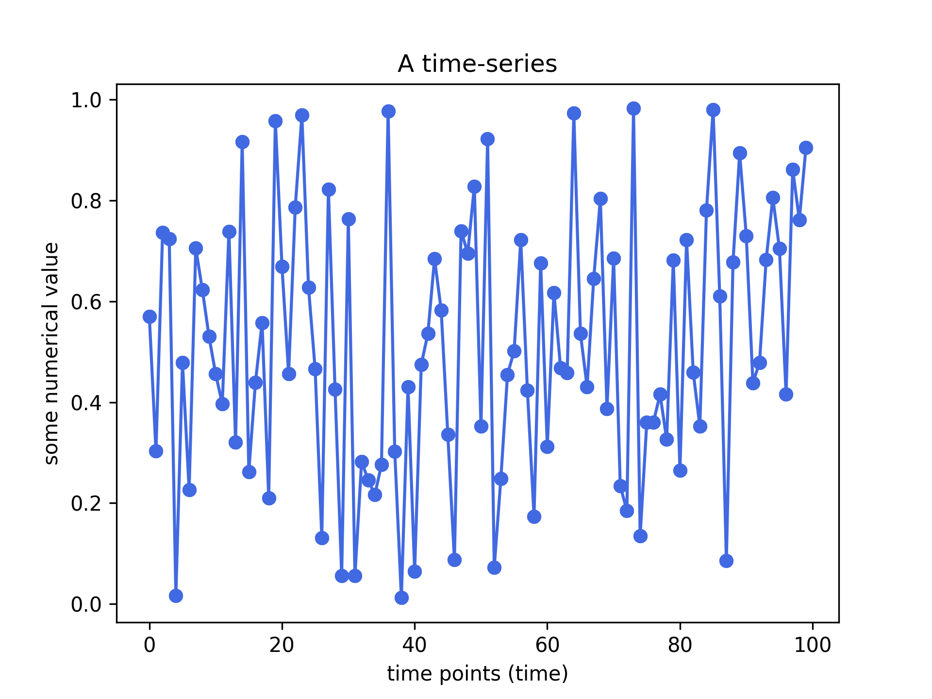
An example of a time-series. Plot created by the author in Python.
Observation: Time-series data is recorded on a discrete time scale.
Disclaimer: There have been attempts to predict stock prices using time series analysis algorithms, though they still cannot be used to place bets in the real market. This is just a tutorial article that does not intent in any way to “direct” people into buying stocks.
2. The AutoRegressive Integrated Moving Average (ARIMA) model
A famous and widely used forecasting method for time-series prediction is the AutoRegressive Integrated Moving Average (ARIMA) model. ARIMA models are capable of capturing a suite of different standard temporal structures in time-series data.
Terminology
Let’s break down these terms:
- **AR: < Auto Regressive > **means that the model **uses the dependent relationship between an observation and some predefined number of lagged observations **(also known as “time lag” or “lag”).
- I:< Integrated > means that the model employs differencing of raw observations (e.g. it subtracts an observation from an observation at the previous time step) in order to make the time-series stationary.MA:
- _MA: < Moving Average > _means that the model exploits the relationship between the residual error and the observations.
Model parameters
The standard ARIMA models expect as input parameters 3 arguments i.e. p,d,q.
- p is the number of lag observations.
- d is the degree of differencing.
- **q **is the size/width of the moving average window.
3. Getting the stock price history data
Thanks to **Yahoo finance **we can get the data for free. Use the following link to get the stock price history of TESLA:
You should see the following:
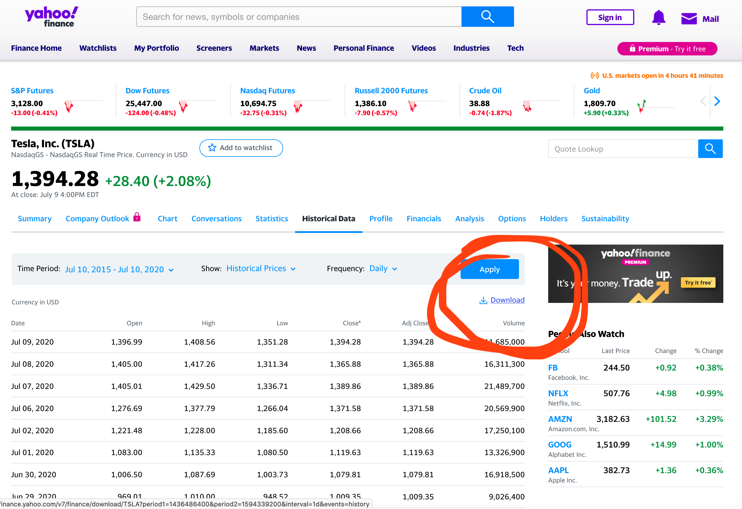
Click on the Download and save the .csv file locally on your computer.
The data are from 2015 till now (2020) !
#time-series-analysis #forecasting #stock-market #data-science #machine-learning #data analysis
